|
|
1.IntroductionWithin the last decade, the use of optical detector arrays with subelectron readout noise has become common for wavefront sensors (WFSs) on astronomical adaptive optics (AO) systems. The majority of these detectors have used electron multiplying charge coupled device (EMCCD) technology,1 for example, as used by the CANARY wide-field AO demonstrator2 on the William Herschel telescope and the SPHERE extreme AO system3 on the very large telescope. However, scientific CMOS (sCMOS) technology4 is now also offering subelectron readout noise and is a potential alternative to EMCCDs, particularly when larger detector arrays are required, for example, for laser guide star (LGS) WFSs and for extremely large telescope scale instruments. An sCMOS camera has been used on-sky by CANARY during LGS commissioning. EMCCD and sCMOS detectors have different readout noise characteristics. The relative effect of different readout noise models on Shack–Hartmann WFS images and the corresponding wavefront slope estimation accuracy have not been previously studied in depth. 1.1.Electron Multiplying Charge Coupled Device Readout NoiseEMCCDs work on the principal of impact ionization, whereas the signals in a given pixel (electrons) are transferred along a many-stage multiplication register; there is a small probability (typically of order 1%, ) that each photoelectron will generate an additional electron. These registers are many hundreds of elements long, and so a large mean multiplication (or gain) can be achieved, equal to where is the number of stages. Unfortunately, this multiplication process is stochastic, and for a given number of input photons in a given pixel, there is a wide range in the possible measured EMCCD output value5 in addition to photon shot noise which is always present. Typically, a gain of order 500 to 1000 is used for astronomical AO systems. After the signal has been multiplied in this way, it is then read out of the detector and digitized, introducing readout noise to the signal. This readout noise is dependent on readout speed and typically has a root mean square (RMS) of about 50 electrons for an EMCCD operated at high-frame rates. We ignore thermal noise, since EMCCDs typically operate at high frame rates and are usually cooled to temperatures of around 220 K in commercial camera models. When modeling the impact of detector performance on instrument designs, the combination of these sources of uncertainty leads to increased complexity. Therefore, simplified models are often used (for example, in Ref. 6): typically, when modeling an EMCCD, the detector quantum efficiency (QE) is halved (i.e., the input flux is halved) as an approximation of the effect of the stochastic gain mechanism, and a readout of around 0.1 electrons is assumed (the true readout noise divided by the gain). Here, we investigate the effect of these assumptions. 1.2.Scientific CMOS Readout NoiseAn sCMOS detector is an active pixel sensor, with each pixel having its own individual readout, rather than a single, or small number of, readout ports as in the case of a CCD. Each sCMOS pixel will, therefore, have an associated readout noise level, which will differ from other readouts due to manufacturing imperfections, etc. Additionally, the readout noise introduced at each pixel will also vary with each frame readout, i.e., the readout noise of a given pixel has some RMS values, with all pixels forming an RMS readout noise probability distribution. Therefore, manufacturers of sCMOS cameras usually quote the median RMS readout of the device, which is at the level of 0.8 electrons for the best current cameras. As with an EMCCD, this level will be dependent on readout speed, which is generally not user-selectable for current commercial sCMOS cameras. Figure 1 shows the histogram of variation of an individual pixel RMS readout for a typical sCMOS device.7 Fig. 1The probability distribution for root mean square (RMS) readout noise of individual scientific CMOS (sCMOS) detector pixels, scaled to the frequency of the modal average. Inset shows the distribution on a logarithmic scale. 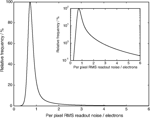 Instrument modeling of sCMOS detectors has to date typically used a single RMS readout value for all pixels (see, for example, Ref. 8), and readout noise is often described using a single (unspecified) parameter, for example, Ref. 9. However, this can lead to an overestimation of instrument performance, since the occasional pixels with far greater readout noise are not modeled. 1.3.Accurate Readout Noise Modeling for Shack–Hartmann Wavefront SensorsThis paper seeks to investigate the effect of accurate readout noise models on the performance of Shack–Hartmann WFSs commonly used for astronomical AO systems. In Sec. 2, we describe the models used, our performance verification, and the implemented tests. In Sec. 3, we discuss our findings and summarize the results. We conclude in Sec. 4. 2.Modeling Readout Noise in Shack–Hartmann Wavefront SensorsTo investigate the effect of sensor readout noise characteristics on Shack–Hartmann WFS performance, we perform Monte-Carlo simulations of a single Shack–Hartmann subaperture, investigating different spot sizes and different subaperture sizes (i.e., number of pixels) for a range of input flux signal levels. Our procedure, following Ref. 6, is as follows:
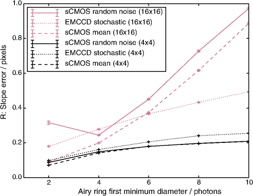
The performance metric is given by where is the ’th individual slope measurement ( or , true or estimated) of Monte-Carlo measurements (typically 10,000). Essentially, this is the mean distance of the estimated position from the true position. We refer to this interchangeably as the slope error (on figure axes) and as the slope estimation accuracy.We use an Airy disk for the noiseless subaperture spot, the width of which is a parameter we investigate (to allow for performance estimates with different pixel scales and seeing conditions), which we define here as the diameter of the first Airy minimum in pixels. When processing the noisy images to compute the spot position, different background levels are subtracted to enable investigation of optimum background subtraction. The background level resulting in the lowest slope error is then used. Signal levels from 20 photons per subaperture (below what would be used effectively on-sky) to 1000 photons per subaperture (approaching a high light level condition) are used. We assume 100% QE for the detectors to simplify data analysis, except for the simplified EMCCD model where the excess noise factor means that the effective QE is 50%.10,11 In practice, the QE of a back-illuminated EMCCD can approach 95%, while second generation sCMOS detectors have a . By scaling flux levels by the relevant QE (as we do in Fig. 14 to provide an example), a reader can evaluate the detector performance for their particular image sensor. Unless stated otherwise, we assume here a spot size of diameter 2 pixels (Airy ring minima), and a signal level of 50 photons per subaperture. We investigate these parameters and the number of pixels within a subaperture. 2.1.EMCCD ModelsWe introduce three models for EMCCD technology readout noise:
For the stochastic and probability distribution models, we use a mean gain of 500 (unless otherwise stated), with 520 multiplication stages, and, thus a probability of about 1.2% of a new electron being generated at each stage for each input electron. We also do not investigate other readout noises, which could be introduced at different detector readout speeds. To achieve the same performance at other readout noise levels, the EMCCD gain could be altered. The probability distribution for EMCCD output is given by Eq. (2), taken from Ref. 5. Additionally, here we also introduce an approximation for this distribution at higher light levels (e.g., for greater than 50 input photoelectrons): And our high light level approximation where is the number of input photo-electrons, is the mean gain, and is the output of the probability distribution. We use the high light-level approximation for input signal levels greater than 50 photoelectrons.2.1.1.Thresholding schemesWe also investigate a thresholding scheme for EMCCD output data, as introduced by Ref. 5. In particular, we use the Poisson probability scheme. This concept involves taking the EMCCD output, dividing by the mean gain, and placing it into nonuniformly spaced bins, with the ’th bin being interpreted as detected photoelectrons. The positions (thresholds) of bin boundaries that we use are given by Ref. 5, placed where the probability of obtaining a given output signal for a light level of photons and photons is equal. This thresholding scheme is nonlinear, and as a result, it does not provide a calibrated flux measurement. Application of a photometric correction is, therefore, also investigated here, as given in Ref. 5. We note that this scheme is far from perfect, as identified in Ref. 11, and so seek only to investigate whether performance improvements are possible when using it. 2.2.Scientific CMOS ModelsWe also introduce a number of models for sCMOS readout noise:
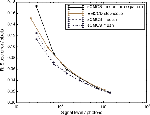
It should be noted that in the cases where the RMS readout noise follows the probability distribution [Eq. (3)], some pixels will have a much larger RMS readout noise than others and thus will have a negative effect on centroid estimates. We use a probability distribution that closely matches manufacturer data,7 given by where is the probability of a given pixel having readout noise and is the normalization factor. Figure 1 shows this distribution. We assume a slow-scan readout scheme to generate this probability distribution: a fast-scan readout would introduce more noise, shifting the distribution.The random nature of pixel RMS readout noise obtained from this distribution means that some subapertures will behave very well (with low noise throughout), while others will contain one or more noisy pixels, particularly for larger subapertures. To get some feel for this effect, we randomly generate noise patterns for 10 different subapertures, which are then used throughout the simulations (and for interest are shown in Fig. 2 for the case). Additionally, to get a better estimate for the “mean” performance of the sCMOS detector, we also include results where a new RMS readout noise pattern was obtained for every Monte-Carlo iteration (using the probability distribution, Fig. 1), the “sCMOS random” model. It is important to note that these readout noise patterns are not a static offset added to the image. Rather, they represent the RMS readout noise of the individual pixels; for each Monte-Carlo iteration, this RMS value is used to generate the particular number of noise electrons introduced, randomly distributed in a Gaussian distribution with a standard deviation equal to the RMS. 3.Implications for Instrumental Modeling of Low-Noise DetectorsThe first question that we seek to answer is the appropriateness of using the simplified EMCCD model for instrument design decisions. Figures 3 and 4 show slope error as a function of signal level for different subaperture sizes, when the different EMCCD readout models are used. It can be seen that the probability distribution model agrees very closely with the full stochastic model. Fig. 3A figure showing slope error as a function of signal level for the different electron multiplying charge coupled device (EMCCD) readout models, as given in the legend. The groups of lines (differentiated by color or shade) represent different subaperture sizes, as given by the annotations on the figure. This figure is for a narrow spot diameter (Airy minimum separated by 2 pixels). 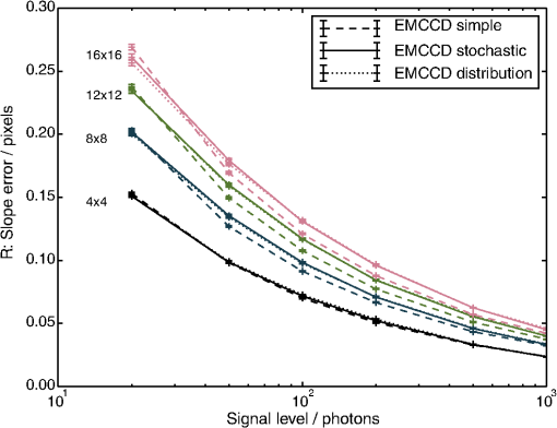 Fig. 4A figure showing slope error as a function of signal level for the different EMCCD readout models, as given in the legend. The groups of lines (differentiated by color or shade) represent different subaperture sizes, as given by the annotations on the figure. This figure is for a wide spot diameter (Airy minimum separated by 10 pixels). 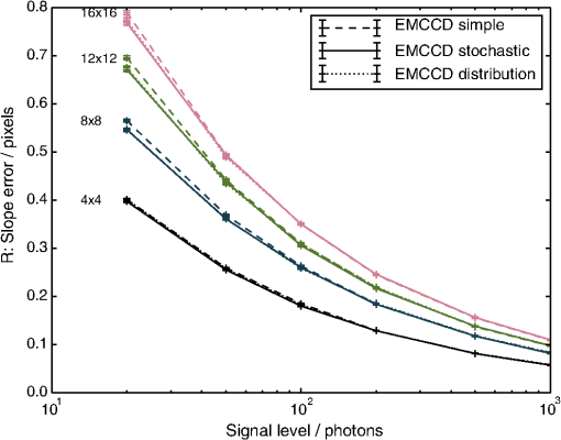 At intermediate flux levels, the simple model slightly underestimates the slope error for small spot sizes (Fig. 3), while there is a slight overestimation of slope error for larger spot sizes (Fig. 4). However, the difference between the simple model and stochastic model is small, and unlikely to be a dominant source of error for AO instrument models. We, therefore, recommend that it is appropriate to use the simple EMCCD model during AO system analysis and design. For astrometry, the case is not so simple. Here, the difference in spot position determination accuracy between the models may be more significant. Therefore, we recommend that design studies for astrometric instruments should at least investigate a full EMCCD stochastic model (or probability distribution model), rather than assuming that the simple model is accurate enough. We discuss this further in Sec. 3.4. 3.1.EMCCD GainThroughout our modeling, we have used a mean EMCCD gain of 500, which is close to the value that we frequently use on-sky with CANARY. However, Fig. 5 also shows the slope estimation error at different levels of mean gain for different light levels. It is clear here that at the lowest light levels, performance predicted by the “EMCCD simple” model is worse than that of other models. We note that at 100 photons per subaperture (and at higher light levels), the “EMCCD simple” model is optimistic. We also note that the “EMCCD stochastic” and “EMCCD distribution” models give almost identical performances. 3.2.Impact of Thresholding SchemesFigure 6 shows the improvement in slope error brought about by thresholding of the EMCCD output for different signal levels, as a function of EMCCD gain, when compared with an unprocessed stochastic multiplication model. It can be seen that by using the thresholding scheme and applying the photometric correction, a reduction in slope estimation error is achievable, reducing the error by up to 5% under certain signal level conditions. We note that the photometric correction is necessary, as applying thresholding without this correction results in poorer performance. The reduction in slope error is at best about 5%, and at the lowest light levels, performance is worse, therefore, we recommend that further investigation is required for a given situation (subaperture size, spot size, etc.) before this strategy should be considered. Fig. 6The improvement in slope estimation accuracy resulting from application of a thresholding scheme as a function of EMCCD gain at different signal levels (as given within the plots), compared to a stochastic multiplication gain model. An improvement is signified by a value greater than unity (the dotted line at unity refers to performance without thresholding). Results with, and without, photometric correction are given, and the subaperture size is , for a spot of diameter 4 pixels (first Airy minimum). 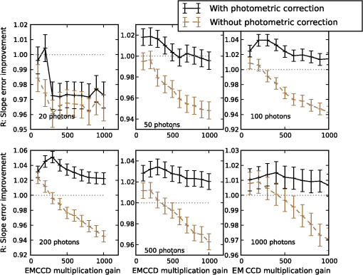 3.3.Scientific CMOS Model ImplicationsThe parameter most commonly given for sCMOS readout noise by camera manufacturers is the median value, which is as low as 0.8 photoelectrons for second generation devices. The RMS readout noise is also sometimes given, with typical values around 1.1 photoelectrons. For instrument design studies, it can be tempting to use either of these values, or something in between, when modeling sCMOS detectors, for example, Ref. 8 use a value of 1 photoelectron as representative of sCMOS readout noise. Here, we compare slope estimation accuracy using both the typical median and mean values, and also using models with interpixel variation in readout noise, following the distribution given in Fig. 1. This probability distribution gives a median readout noise of 0.8 photoelectrons and a mean of 1.08. Figure 7 shows slope estimation accuracy comparing these different models when large subapertures () are used. The EMCCD stochastic model performance is also shown for comparison. It is interesting to note that using the median and mean sCMOS models provides a significantly better performance than the EMCCD model. At first sight, if one of these simple sCMOS models is used during instrument development, then it will appear that sCMOS technology is more appropriate for Shack–Hartmann wavefront sensing than EMCCD technology. However, once the probability distribution for readout noise is taken into account, this is clearly no longer the case. As Fig. 7 shows, true sCMOS performance is significantly worse than the predicted performance using the simple models. Fig. 7A figure showing slope estimation error as a function of signal level for different detector readout models, for a subaperture with . 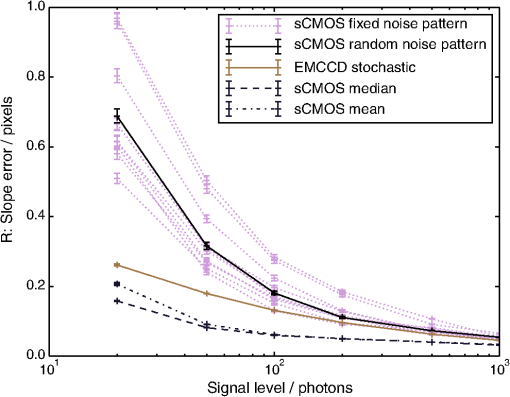 3.3.1.Spread of subaperture performanceThe 10 curves for subapertures with different fixed readout noise patterns in Fig. 7 show a significant spread in slope error. This is because some of these subapertures are “unlucky” (Fig. 2), in that they contain one or more pixels with readout noise in the tail of the probability distribution (Fig. 1). Even the “lucky” subapertures, which yield the lowest slope error, still have performances significantly worse than simple readout models predict, and still significantly worse than the EMCCD performance. This is because the pixels within these subapertures still have a range of readout noise levels (the highest noise pixel in the best subaperture having a readout noise of 5.95 electrons, and the highest noise pixel in the worst subaperture having a readout noise of 9.34 electrons). To get an idea of the “average” expected performance using a sCMOS detector, the “sCMOS random” model was used: for every Monte-Carlo iteration, each pixel is assigned a new RMS readout noise from the probability distribution. This RMS readout noise is then used to obtain the number of readout electrons introduced with that iteration, using a Gaussian distribution with a standard deviation equal to the RMS. In effect, this allows us to sample an average performance over a large number of subapertures, and the results are given by the “sCMOS random noise pattern” curve in Fig. 7. It can be seen here that this offers significantly worse slope estimation accuracy than either the EMCCD or simple sCMOS models. Currently, available sCMOS detectors have large pixel counts. Therefore, for applications requiring low-order wavefront sensing, where fewer pixels are required, it may be possible to select an area of the sCMOS detector where the RMS readout noise is generally low. However, this will be device dependent, and we do not consider it further here. 3.3.2.Performance dependence on subaperture sizeFigure 8 shows the slope estimation accuracy for different detector readout models on a subaperture. For all but the lowest light levels, the “average” expected performance using the sCMOS detector (the “sCMOS random” model) is better than that of the EMCCD. It is interesting to note that some subapertures are “lucky,” with a performance at the level of that predicted by simple sCMOS models (i.e., constant readout noise equal to median or mean). This is because, with far fewer pixels, there is a higher probability that all pixels within a subaperture can avoid the tail of the probability distribution. Of the 10 subaperture readout noise patterns used, the maximum RMS readout noise varied between 0.94 (for the best subaperture) and 7 electrons (for the worst). The mean RMS values ranged from 0.72 to 1.3 electrons. Fig. 8A figure showing slope estimation error as a function of signal level for different detector readout models, for a subaperture with . 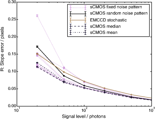 Figure 9 shows slope estimation accuracy as a function of subaperture size. It can be seen that the EMCCD performance is better than the sCMOS performance for subaperture sizes equal to and greater than . For comparison, the simple sCMOS model results are also provided and show that performance will be greatly overestimated if these models are used. Fig. 9A figure showing slope estimation error as a function of subaperture size for different detector readout models as given in the legend. The subaperture size refers to the linear dimension, i.e., the square root of the total number of pixels within a subaperture. 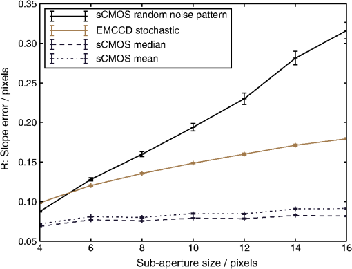 Therefore, we recommend that proper models of sCMOS readout noise should always be used when modeling instrument performance. 3.3.3.Performance dependence on spot sizeFigure 10 shows slope estimation accuracy as a function of Shack–Hartmann spot size. For smaller subapertures, the sCMOS performance is better than the EMCCD performance. However, for larger subapertures, the EMCCD performance is generally better, particularly as spot size increases (with the available flux being spread over more pixels). We note that the performance of the sCMOS technology predicted using the full noise distribution model is always significantly worse than performance predicted using a simple (constant RMS readout noise) model for larger subapertures. 3.3.4.Simple model for scientific CMOS readout noiseWe have established that using the mean or median sCMOS RMS readout noise when estimating instrumental performance is optimistic. Unfortunately, using a full probability distribution will introduce additional complexity to instrumental modelling and increase the parameter space that requires exploration, in part due to the need to randomly sample different parts of the probability distribution (to sample different areas of a detector) to obtain an average expected performance. Therefore, if a single-parameter model sCMOS readout noise can be obtained, this will greatly simplify instrumental modeling. Figure 11 compares the slope estimation error () for different readout noise models. These include the 10 “sCMOS fixed” models identified earlier (e.g., Fig. 2), the “sCMOS random” model, and also models with a range of constant RMS readout noise values. By comparing the “sCMOS random” model with the closest constant RMS model for a given signal level, we can get a feel for the “effective” readout noise of the detector for that particular case. Fig. 11A figure showing slope estimation error as a function of signal level for different sCMOS readout noise models, for a (a) and (b) pixel subaperture. The dashed lines show the slope error predicted using a constant RMS readout noise, the value of which is given adjacent to the lines. The solid line shows the average expected slope area from a sCMOS detector (the “sCMOS random” model). The dotted lines represent the “sCMOS fixed” model and are shown to give an idea of spread in performance. 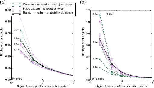 To make sense of this information and to provide a useful reference for future instrument modelling, Fig. 12 shows the single-value RMS readout noise that will provide the same performance as predicted by the “sCMOS random” model, for different subaperture and spot sizes. To use this figure when modeling a specific AO instrument, the known subaperture and spot size can be used to read off an effective RMS Gaussian readout noise for an sCMOS detector on the figure, i.e., a single readout value for the detector. This effective RMS Gaussian readout noise can then be used to predict AO system performance, giving a similar result as that expected if the full randomly sampled RMS readout noise probability distribution had been used, but with reduced complexity. Fig. 12A figure showing the effective Gaussian sCMOS RMS readout noise that predicts the same slope estimation performance as that predicted by random sampling of the RMS readout noise probability distribution. Values are given as a function of subaperture size and spot diameter (Airy ring first minimum diameter). Six different signal levels are shown, with the number of photons per subaperture given inset in the figures. 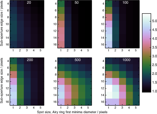 It is important to note that different sCMOS detector generations and chip sizes will have a different RMS readout noise probability distribution. We, therefore, recommend that an equivalent to Fig. 12 should be generated for the specific detector family under consideration in an instrument design. Using this information will allow a more accurate prediction of instrumental performance to be made. 3.3.5.Elongated spots for laser guide starsSo far, we have only considered Shack–Hartmann point spread functions (PSFs) with circular symmetry. However, it is also important to consider the case when extended LGS sources are used, producing elongated PSFs. Figure 13 shows slope estimation error as a function of elongation for a subaperture. A two-dimensional Gaussian model has been used for the LGS spot PSF, with the Gaussian standard deviation in one dimension investigated. We note that using a standard deviation of unity gives a spot of size broadly equivalent to an Airy disk with the diameter of the first minimum being six pixels. We apply the different readout noise models to these elongated spots, as described previously. Fig. 13A figure showing slope estimation error as a function of LGS elongation, with the relevant elongated spot PSFs shown inset ( subapertures). The different detector readout noise models are given in the legend. Ten different fixed-pattern sCMOS RMS readout noise patterns are shown undifferentiated, to give an idea of the spread in performance due to the random nature of the readout noise probability distribution. 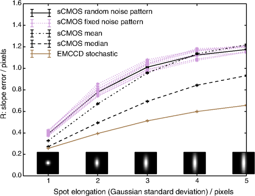 It can be seen that EMCCD technology provides the lowest error. All three EMCCD readout noise models predict very similar performances, thus only the “EMCCD stochastic” model is shown for clarity. It is interesting to note that as the spot becomes more elongated, the sCMOS performance predicted using the “sCMOS mean” model becomes closer to that predicted by the “sCMOS random” model, thus suggesting that a simple model for sCMOS readout noise is applicable for elongated LGS spots. We note that in a real AO system, the degree of LGS elongation will depend on subaperture position within the telescope pupil, and some subapertures will remain almost unelongated. In this case, the simple sCMOS readout noise model is optimistic, and so we recommend that a full sCMOS readout noise model based on the RMS readout noise probability distribution should be used whenever readout noise is a key instrument design consideration. 3.3.6.Considerations of quantum efficiencyWe have so far ignored detector QE and assumed identical QE for all detector models (though we halve the effective QE for the simple EMCCD model). The QE of EMCCD devices can reach 95% (e.g., the Andor iXon3), while for sCMOS detectors, it is closer to 70% (e.g., the Andor Zyla 4.2). Figure 14 shows the slope estimation error once the QE is taken into account and can be compared directly with Fig. 8 (which assumes identical QEs). It can be seen here that EMCCD performance is now at least as good as that predicted by the “sCMOS random” model, i.e., in practice, an EMCCD detector is likely to perform as well as a sCMOS detector for subapertures (and, as we have seen previously, better for larger subapertures). 3.4.Astrometric AccuracyWe have investigated the effect of detector readout noise models on image centroiding accuracy. In addition to importance for AO systems, accurate position determination is critical for astrometric techniques. We have shown that there are only small differences in estimation accuracy between the commonly used simple EMCCD model and a full stochastic gain mechanism model. However, for some astrometric observations, this difference may be critical, therefore, we recommend that the full stochastic gain mechanism (or the EMCCD output probability distribution model, which is almost identical) should be used, until it can be demonstrated that the simple model is sufficient for each particular instrument study. We note here that the stochastic model is computationally more expensive than other models. When using sCMOS technology for astrometric applications, greater care is required. We have shown that a simple model of sCMOS readout noise based on a single RMS value for all pixels (whether the median or mean) is optimistic. Therefore, a model for sCMOS readout noise that uses the per-pixel probability distribution for RMS noise is essential. Further model improvements can be made if the precise RMS readout noise pattern for a physical detector under consideration can be used (i.e., once the detector has been acquired), though we do not consider this further here. 4.ConclusionsWe have investigated detector readout models for sCMOS and EMCCD technologies and the effect that these models have on slope estimation accuracy for Shack–Hartmann WFSs used in AO systems. Our findings are also relevant to any problem involving image center of mass location, including astrometry. We find that, in general, EMCCD technology offers better performance than sCMOS technology for Shack–Hartmann WFSs and other applications requiring center of mass calculations. We find that the commonly used simple model for EMCCD readout (halving the effective QE and assuming a subelectron readout noise) is sufficient for AO applications with a predicted slope estimation accuracy differing only slightly from when using a full Monte-Carlo stochastic gain mechanism model. A model based on the EMCCD probability output distribution also performs almost identically to the stochastic gain model. For sCMOS technology, we find that the commonly used model that uses a single RMS readout value for all pixels (whether the median or mean) produces optimistic results, which can predict a better performance than that obtained by EMCCD detectors. However, more reliable performance estimates during instrument development and design studies can be made by taking a typical sCMOS RMS readout noise probability distribution into account, and we find that this model generally predicts a worse performance than that obtained by EMCCD detectors. Ideally, many random samples of this distribution should be taken, so that an average (and worst case) performance estimate for sCMOS technologies can be obtained. A key finding is that using the median or mean sCMOS RMS readout noise value is not sufficient to accurately predict instrumental performance: the full probability distribution for sCMOS readout noise should be used. AcknowledgmentsThis work is funded by the UK Science and Technology Facilities Council, Grant No. ST/I002871/1 and ST/L00075X/1. ReferencesP. Jerram et al.,
“The LLCCD: low-light imaging without the need for an intensifier,”
Proc. SPIE, 4306 178
–186
(2001). http://dx.doi.org/10.1117/12.426953 Google Scholar
R. M. Myers et al.,
“CANARY: the on-sky NGS/LGS MOAO demonstrator for EAGLE,”
70150E
(2008). http://dx.doi.org/10.1117/12.789544 Google Scholar
T. Fusco et al.,
“High-order adaptive optics requirements for direct detection of extrasolar planets: application to the SPHERE instrument,”
Opt. Express, 14 7515
–7534
(2006). http://dx.doi.org/10.1364/OE.14.007515 OPEXFF 1094-4087 Google Scholar
C. Coates, B. Fowler and G. Holst,
“Scientific CMOS technology: a high-performance imaging breakthrough,”
(2015) http://www.scmos.com/files/low/scmos_white_paper_2mb.pdf February ). 2015). Google Scholar
A. G. Basden, C. A. Haniff and C. D. Mackay,
“Photon counting strategies with low-light-level CCDs,”
Mon. Not. R. Astron. Soc., 345 985
–991
(2003). http://dx.doi.org/10.1046/j.1365-8711.2003.07020.x Google Scholar
A. G. Basden et al.,
“Sensitivity improvements for Shack-Hartmann wavefront sensors using total variation minimization,”
Mon. Not. R. Astron. Soc., 449 3537
–3542
(2015). http://dx.doi.org/10.1093/mnras/stv617 Google Scholar
, “pco.edge 4.2 scientific CMOS camera,”
http://www.pco.de/fileadmin/user_upload/pco-product_sheets/BR_pco_edge42_108_online.pdf Google Scholar
A. G. Basden,
“Visible near-diffraction limited lucky imaging with full-sky laser assisted adaptive optics,”
Mon. Not. R. Astron. Soc., 442 1142
–1150
(2014). http://dx.doi.org/10.1093/mnras/stu941 Google Scholar
P. Qiu et al.,
“Evaluation of a scientific CMOS camera for astronomical observations,”
Res. Astron. Astrophys., 13 615
–628
(2013). http://dx.doi.org/10.1088/1674-4527/13/5/012 1674-4527 Google Scholar
M. S. Robbins and B. J. Hadwen,
“The noise performance of electron multiplying charge-coupled devices,”
IEEE Trans. Electron Devices, 50 1227
–1232
(2003). http://dx.doi.org/10.1109/TED.2003.813462 Google Scholar
O. Daigle, C. Carignan and S. Blais-Ouellette,
“Faint flux performance of an EMCCD,”
Proc. SPIE, 6276 62761F
(2006). http://dx.doi.org/10.1117/12.669433 PSISDG 0277-786X Google Scholar
Biography |


