Methods and limitations of focal plane sensing, estimation, and control in high-contrast imaging

Tyler D. Groff; A. J. Eldorado Riggs; Brian Kern; N. Jeremy Kasdin

doi:10.1117/1.JATIS.2.1.011009

17 December 2015 Methods and limitations of focal plane sensing, estimation, and control in high-contrast imaging

Tyler D. Groff, A. J. Eldorado Riggs, Brian Kern, N. Jeremy Kasdin

Journal of Astronomical Telescopes, Instruments, and Systems, Vol. 2, Issue 1, 011009 (December 2015). https://doi.org/10.1117/1.JATIS.2.1.011009

Abstract

Coronagraphy is a very promising method for directly imaging exoplanets, but the performance of a coronagraph is highly sensitive to quasi-static aberrations within the telescope. The resultant speckles are suppressed in the final focal plane using a wavefront control system that estimates the field at the final focal plane to avoid any noncommon path error. This requires a set of probe images that modulate the field so that it may be estimated. With an estimate of the focal plane electric field, a control law is defined to suppress the speckle field so that the planet can be imaged. Characterizing the planet requires that the speckle field be suppressed simultaneously over the bandpass of interest. The choice of control law, bandpass, estimator, and probing methodology has implications in the control solutions and contrast performance. Here, we compare wavefront probing, estimation, and control algorithms, and describe their practical implementation.

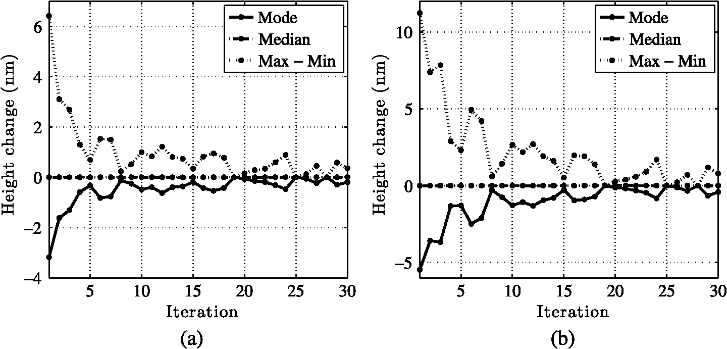
1. Introduction

Directly imaging exoplanets, particularly Earth-like exoplanets, has been a goal of the scientific community for some time and was identified as a key technological priority in the last decadal review.¹ Starshades and coronagraphs are the key enabling technologies for direct imaging missions in space. Both are experiencing great successes in their technology development, with a few modern examples of these designs being the Exo-S,² Exo-C,³ and WFIRST-AFTA⁴ studies. The starshade option requires formation flight of the telescope with a second satellite that occults the star to a diffraction-limited level so that only the planet light enters the telescope. A coronagraph relies on a series of apodizers, masks, and stops in the instrument to suppress the starlight so that the off-axis planets can be imaged. The trade for a single satellite means that the starlight enters the telescope, resulting in aberrations that leak starlight into the coronagraphic image. Even small aberrations affect contrast at a $10^{- 10}$ contrast level, the relative intensity at which we expect to see Earth-like exoplanets. Furthermore, these aberrations are dynamic in even the most stable telescope and result in a quasi-static speckle field in the image plane. The solution is to include deformable mirrors in the instrument so that the resultant speckles can be actively suppressed, allowing us to recover a dark hole of high contrast in the image plane. The precision required to create a dark hole at extremely high contrast drives wavefront-sensing methods away from sensors that introduce noncommon path optics. Thus, the control loop is closed around the final science image where we must first estimate and then control the electric field to maintain a dark hole in which we can discover and spectrally characterize targets.

Here, we describe the current control and estimation methods for focal plane wavefront control at multiple facilities, most specifically drawn from practical experience at the Princeton University High Contrast Imaging Laboratory (HCIL) and the Jet Propulsion Laboratory’s (JPL) High Contrast Imaging Testbed (HCIT). We begin by formulating the linear problem under the framework of Fourier optics, a common approach to all such focal plane methods. A comparison of the mathematical basis for various controllers and estimators follows. Finally, we describe several probing methods, evaluate the quality of our observation as a function of the probe chGoice, and examine how this affects our ability to achieve high contrast.

2. Wavefront Control

We begin by deriving the underlying mathematics for a generalized focal plane wavefront control instrument. A schematic of the Princeton HCIL layout is given in Fig. 1 to illustrate the concept. One can consider the fiber launch in Fig. 1 to be the input image from the telescope. What follows is the simplest possible control system with two deformable mirrors (DMs). The beam is collimated by an off-axis parabola (OAP), reflects off two DMs in series, and propagates through the apodizer. In the case of the HCIL, the apodizer is a shaped pupil coronagraph,⁵^,⁶ but the choice of apodizer only affects the transformation required to reach the image plane (which is generalized in this paper). With the shaped pupil located in the first pupil plane, we then form the first image with a second OAP, block the core of the point spread function (PSF) with a focal plane mask, and reimage onto the science camera. Note that there is no wavefront sensor, and the purpose of this section is to derive the transformations that describe the effect of perturbations in collimated space on the image plane electric field so that we can ultimately define model-based estimators and control laws where the sensing is done in the image plane. Augmenting the controller to multiple DMs, and mathematically correcting for moving DM surfaces to planes nonconjugate to the pupil is fully described by Pueyo et al.,⁷ with various details of controllability addressed by Shaklan and Green⁸ and Groff.⁹ Once again, these will have small effects on the form of the transformations that we have generalized here.

Fig. 1

Optical layout of the Princeton High Contrast Imaging Laboratory (HCIL). Collimated light is incident on two deformable mirrors (DMs) in series, which propagates through a shaped pupil, the core of the point spread function is removed with an image plane mask, and the 90 deg search areas are reimaged on the final camera when using the Ripple3 shaped pupil coronagraph.

Treating the designed pupil field as $A (u, v)$ , the DM surface as a phase perturbation at the pupil plane, $φ (u, v)$ , and including a distribution of complex aberrations, $g (u, v)$ , the electric field at the pupil plane at any control step $k$ is given by

Eq. (1)

E_{pup, k} (u, v) = A (u, v) [1 + g (u, v)] e^{i φ_{k} (u, v)} .

For controller design, we write the controlled phase at step

k

as a sum of the previous DM surface and a small perturbation,

δ φ

, about which we will ultimately linearize the phase induced by the DM. It is important to note that we show the aberrated field as a separate additive complex error,

g (u, v)

, but this makes it less obvious that the initial field about which one linearizes should be the entire phase distribution in the pupil. In other words,

φ_{0} (u, v)

would include an estimate of the entire aberrated field. At HCIT, this comes from the initial phase diversity estimates used to flatten the pupil field and determine its starting complex field.

Assuming that the phase perturbation from the DM, $δ φ_{k}$ , is adequately small, we let $φ_{k} = φ_{k - 1} + δ φ_{k}$ and take a first-order approximation of the exponential, resulting in the linearized form of the pupil field.

Eq. (2)

E_{pup, k} (u, v) ≅ A (u, v) [1 + g (u, v)] e^{i φ_{k - 1}} [1 + i δ φ_{k} (u, v)] .

Additionally, we assume that the product

g δ φ_{k}

is negligible compared to the other terms since they will both be small and are of approximately the same magnitude, letting us rewrite the expanded field as

Eq. (3)

E_{pup, k} (u, v) ≅ A (u, v) e^{i φ_{k - 1}} [1 + g (u, v) + i δ φ_{k} (u, v)] .

Treating the propagation through the coronagraph and imaging system as a linear transformation between the image and pupil planes,

C {\cdot}

, the linearized form of the image plane electric field is written as

Eq. (4)

E_{i m, k} (x, y) = C {A (u, v) e^{i φ_{k - 1}} [1 + g (u, v)]} + i C [A (u, v) e^{i φ_{k - 1}} δ φ_{k} (u, v)] .

Wavefront control is accomplished by commanding DM actuators, not setting the phase across a mirror. Thus, we apply a physical model of the DM in terms of actuator commands. Normalizing the surface height of the mirror,

H (u, v)

, by the wavelength,

λ

, the phase shift,

φ (u, v)

, induced by the DM is given by

Eq. (5)

φ (u, v) = \frac{4 π}{λ} H (u, v) .

We describe this surface profile as a combination of the two-dimensional height maps imposed by each actuator. Since we are using a DM with a continuous face sheet, the contribution of any actuator will be highly localized but will still deform the entire DM surface. Thus, we define the contribution of any

q

’th actuator as a characteristic two-dimensional phase map over the entire plane of the DM surface with unitary amplitude,

f_{q} (u, v)

. We can then describe

H (u, v)

as a superposition of these characteristic shapes, commonly referred to as influence functions, over all

N_{act}

actuators. Defining the amplitude of each influence function (represented as a phase shift in meters to eliminate a factor of two) as

a_{q}

, the phase perturbation induced by the DM becomes

Eq. (6)

φ (u, v) = \frac{2 π}{λ} \sum_{q = 1}^{N_{act}} a_{q} f_{q} (u, v) .

Since Eq. (6) is linear in actuator amplitudes, we can substitute Eq. (6) for

δ φ_{k}

in Eq. (4). The image plane response to a change in actuator amplitudes at the

k

’th step is given by

Eq. (7)

E_{i m, k} (u, v) = C {A (u, v) e^{i φ_{k - 1}} [1 + g (u, v)]} + \frac{2 π i}{λ} \sum_{q = 1}^{N_{act}} δ a_{q} C [A e^{i φ_{k - 1}} f_{q} (u, v)] .

Since we only measure the field intensity at a finite number of pixels, we convert the continuous functions in Eq. (7) to values at each pixel and rewrite in matrix form.

Eq. (8)

E_{i m, k} = C [A e^{i φ_{k - 1}} (1 + g_{k})] + G_{k} u_{k},

where

E_{i m, k}

is a matrix of dimension

N_{pix} \times 1

containing the electric field at each pixel.

Eq. (9)

G_{k} = i C (A e^{i φ_{k - 1}} f)

is the

N_{pix} \times N_{act}

control effect matrix accounting for the propagation of each influence function, each of which is embedded in a matrix

f

, and

u_{k}

is a column matrix of changes in actuator amplitudes at step

k

,

u_{k} = {[δ a_{1} \dots δ a_{N_{act}}]}_{k}^{T}

. The discretization of the field is naturally subject to numerical effects. One must take care to correctly sample each plane, and the choice of transform method can also become important. Numerical transforms are widely used in high-contrast imaging experiments, and their effect has been well studied. One notable study was done in the development of the PROPER optical propagation library by Krist.¹⁰

Finally, the measured intensity in the image plane is just the square of the field, $I_{i m, k} (x, y) = {| E_{i m, k} (x, y) |}^{2}$ . We often refer to the area in the image plane where sufficient contrast has been achieved as the dark hole and use the notation $I_{DH}$ for the high-contrast intensity (either designed or controlled) there. The objective of the wavefront controller is to find the control matrix $u_{k}$ that will recover the desired contrast in the dark hole in the presence of the aberrations.

3. Speckle Nulling

Speckle nulling, whose fundamental equations are described fully in Ref. 11 along with a speckle energy minimization and sensing scheme, is the simplest form of suppression in the final image plane. It does not require an estimate of the electric field and, therefore, only closes the loop on intensity images in an attempt to slowly drive the unobservable field states to zero. All that is needed is a mapping of spatial frequencies at the DM plane to image plane locations. Speckles are then singled out in the image and suppressed based on their intensity and phase. The amplitude of the command for any spatial frequency is directly proportional to the intensity of the speckle. Specifically, the DM amplitude should scale as $λ \sqrt{I_{speckle}}$ . The correct phase shift for each spatial frequency command on the DM is determined by minimizing the energy of the speckle in the image plane. Since the amplitude and phase of any spatial frequency on the DM are computed directly from intensity measurements at the detector, speckle nulling tends to be highly robust to model error and does not require as much computational overhead. However, it is highly inefficient compared to other control methods because speckles are dealt with one at a time and there is no guarantee that canceling a speckle will not degrade the contrast of other speckles. This has been mitigated in some sense by simultaneously solving for the multiple speckles at a time, which has been reported at the Ames Coronagraph Experiment Laboratory, where the algorithm is typically used in conjunction with electric field conjugation (EFC).¹² Despite this, speckle nulling tends to be slow and is largely relied upon to clean up stray artifacts. The main advantage of speckle nulling is its robustness to model error, which is thoroughly demonstrated on sky by Martinache et al. without the aid of extreme adaptive optics.¹³

4. Monochromatic Model–Based Control Algorithms

The primary control laws used in focal plane wavefront control for the past decade at Princeton and JPL are stroke minimization⁷ and EFC.¹⁴ Though other variants, such as the coronagraphic focal plane wavefront estimation for exoplanet detection (COFFEE)¹⁵ algorithm, have also been studied, stroke minimization and EFC have achieved the highest contrast of any controllers to date and are the primary control laws under consideration for the WFIRST-AFTA coronagraph system. In this section, we describe each, highlighting their differences and similarities.

4.1.

Stroke Minimization—Lagrange Multipliers

The stroke minimization algorithm⁷ seeks to regularize the control solution by directly minimizing stroke under the constraint that the solution for the desired DM perturbation achieves a specified contrast level.

Applying the matrix form of the control amplitudes in Eq. (9) and taking the inner product (represented as $⟨ \cdot, \cdot ⟩$ ) of Eq. (4), we find the intensity in the dark hole at the operation wavelength, $λ_{0}$ , to be

Eq. (10)

I_{DH} (k) = \frac{4 π^{2}}{λ_{0}^{2}} u_{k}^{T} M_{k} u_{k} + \frac{4 π}{λ_{0}} u_{k}^{T} I {b_{k}} + d_{k},

where

I {\cdot}

is the imaginary component of the operand, and

Eq. (11)

M_{k} = ⟨ C (A e^{i φ_{k - 1}} f_{k}), C (A e^{i φ_{k - 1}} f_{k}) ⟩ = G_{k}^{*} G_{k},

Eq. (12)

b_{k} = ⟨ E_{a b, k}, C (A e^{i φ_{k - 1}} f_{k}) ⟩ = G_{k}^{*} E_{a b, k},

Eq. (13)

d_{k} = ⟨ E_{a b, k}, E_{a b, k} ⟩ = E_{a b, k}^{*} E_{a b, k},

Eq. (14)

E_{a b, k} = C [A e^{i φ_{k - 1}} (1 + g_{k})] .

Conceptually,

d_{k}

is the column matrix of the intensity contribution from the aberrated field,

E_{a b, k}

. The measured intensity can be used to construct

d_{k}

if there is not a large bias in the signal. The matrix

b_{k}

represents the interaction of the DM electric field with the aberrated field, and

M_{k}

describes the additive contribution of the DM to the image plane intensity for a given DM shape,

f_{k}

, at control step

k

. Having represented

I_{DH}

in a quadratic form in terms of the control signal, we can use Eq. (10) to produce an optimal control strategy. The optimization problem in monochromatic light is functionally stated as

Eq. (15)

\begin{array}{l} minimize & \sum_{q = 1}^{N} a_{q, k}^{2} = u_{k}^{T} u_{k} \\ subject to & I_{DH} (k) \leq C_{k} \end{array},

where

C_{k}

is the contrast constraint at each iteration, which changes over time to steadily decrease contrast.

To solve the optimization problem, Pueyo et al.⁷ realized a control law by modifying the inequality constraint in Eq. (15) to be represented as the equality constraint $(I_{DH} - C_{k}) = 0$ . Incorporating the equality constraint for the central wavelength into the minimization on stroke via a Lagrange multiplier, $μ_{k}$ , yields a quadratic cost function given by

Eq. (16)

J_{k} = u_{k}^{T} u_{k} + μ_{k} [I_{DH} (k) - C_{k}] = u_{k}^{T} u_{k} + μ_{k} (\frac{4 π^{2}}{λ_{0}^{2}} u_{k}^{T} M_{k} u_{k} + \frac{4 π}{λ_{0}} u_{k}^{T} I {b_{k}} + d_{k} - C_{k}) = u_{k}^{T} (I + μ_{k} \frac{4 π^{2}}{λ_{0}^{2}} M_{k}) u_{k} + μ_{k} \frac{4 π}{λ_{0}} u_{k}^{T} I {b_{k}} + μ_{k} (d_{k} - C_{k}),

where

I

represents the identity matrix. The quadratic form guarantees a single minimum to the linearized equation. This is identical to a linear least squares solution. Recognizing that

M_{k}

is guaranteed to be symmetric, and hence

M_{k} = M_{k}^{T}

, we take the partial derivative to find actuation that minimizes the cost function. Evaluating

Eq. (17)

\frac{\partial J}{\partial u_{k}^{T}} |_{u_{J, k}} = 2 (I + μ_{k} \frac{4 π^{2}}{λ_{0}^{2}} M_{k}) u_{J, k} + μ_{k} \frac{4 π}{λ_{0}} I {b_{k}} = 0

and solving for the optimal control input, we find

Eq. (18)

u_{J, k} = - {(\frac{1}{μ_{k}} \frac{λ_{0}}{2 π} I + \frac{2 π}{λ_{0}} M_{k})}^{- 1} I {b_{k}} .

To find the value of

u_{J, k}

, all that is left is to find the value of

μ_{k}

that minimizes the cost function, Eq. (16). This has historically been done via a line search on

μ_{k}

, continuously increasing

μ_{k}

, evaluating

u_{k}

with Eq. (18) for each value of

μ_{k}

until the quadratic intensity given by Eq. (10) goes below the targeted contrast value. Since this is a linearized subprogram, we must relinearize about the new DM shape at each iteration of the correction algorithm (or every time we apply a new DM command). This is computationally expensive, so we tend not to do this in the experiment. However, the nature of the controller is such that the solution will not deviate dramatically from the optimal one found by relinearizing at each iteration. Since the controller is trying to minimize stroke, the control signal tends to remain in the regime of a particular linearization for as long as possible. Statistics on the control history for a representative two-DM experiment at HCIL is shown in Fig. 2. We observe that the vast majority of stroke is used to eliminate strong aberrations in the first five iterations of the control history. After this, the extrema and mode reduce dramatically, frequently a factor of 10 less stroke than the first iteration. Throughout the entire control history, the median never deviates far from zero, meaning that a dc drift never develops and the shape about which we are linearizing is nearly identical as we approach our ultimate achievable contrast.

Fig. 2

Time history of actuation statistics for each DM. We plot the mode, median, and peak-to-valley actuation levels for (a) DM1 and (b) DM2 in a representative control run at the Princeton HCIL. The starting contrast is $1 \times 10^{- 4}$ and final contrast is $2.3 \times 10^{- 7}$ in symmetric dark holes.

4.2.

Electric Field Conjugation—Tikhonov Regularization

EFC is an alternate controller approach first presented by Give’on et al.¹⁴ It was originally modeled on the traditional, pupil-based adaptive optics approach, where the DM is set to conjugate the phase in the pupil to recover as flat an entering field as possible. In focal plane wavefront control, the analogous field conjugation would be done in the image. That is, given an estimate of the electric field at step $k - 1$ from Eq. (8), ${\hat{E}}_{i m, k} = C (\hat{A e^{i φ_{k - 1}}}) + C (\hat{A e^{i φ_{k - 1}}} g)$ , the EFC controller seeks to drive to a desired field, $E_{D}$ , allowing us to define the targeted field perturbation as

Eq. (19)

δ E_{k} = {\hat{E}}_{i m, k} - E_{D} .

Substituting for the control effect in Eq. (8), the goal is to use the DM to create a field perturbation,

δ E_{k}

, such that the desired field becomes

Eq. (20)

E_{D} = C {A (u, v) e^{i φ_{k - 1}} [1 + g (u, v)]} + δ E_{k} . = E_{i m, k} (x, y) .

In its original form, EFC seeks to find a control $G_{k} u_{k}$ that conjugates the residual aberration terms in Eq. (20), to create the desired final field in the image plane. The effect of different choices of $E_{D}$ will become clearer once the controller has been fully defined.

Unfortunately, given the limitations of the influence function form of the DMs, the image plane field perturbation in Eq. (20) is not always reachable. In other words, one cannot simply invert $G_{k}$ to solve for $u_{k}$ given the desired field perturbation defined in Eq. (19). Instead, EFC seeks to find a control as close to the desired field perturbation as possible. We do so by defining an error, $ϵ_{k}$ , between the controlled field and the desired field as

Eq. (21)

ε_{k} = G_{k} u_{k} - δ E_{k} .

EFC seeks to minimize this error rather than minimize the stroke as in Sec. 4.1. Doing so via a simple least-squares solution, however, often produces an ill-posed problem. Thus, EFC uses a regularized cost function to guarantee inversion. The regularization parameter,

Γ_{k}

, is introduced via a Tikhonov regularization, making the quadratic cost function

Eq. (22)

W_{k} = {(G_{k} u_{k} - δ E_{k})}^{*} (G_{k} u_{k} - δ E_{k}) + u_{k}^{T} Γ_{k}^{T} Γ_{k} u_{k} .

Evaluating the partial derivative,

Eq. (23)

\frac{\partial W_{k}}{\partial u_{k}} |_{u_{w, k}} = 2 (G_{k}^{*} G_{k} + Γ_{k}^{T} Γ_{k}) u_{w, k} - 2 G_{k}^{*} δ E_{k} = 0,

the control vector that minimizes Eq. (22),

u_{w, k}

, is given by

Eq. (24)

u_{w, k} = {(G_{k}^{*} G_{k} + Γ_{k}^{T} Γ_{k})}^{- 1} G_{k}^{*} δ E_{k} .

With no particular reason to weight any specific field position or actuator, the regularization matrix,

Γ_{k}

, is defined as

Eq. (25)

Γ_{k} = α_{k} I .

The regularized solution and its associated cost are then given by

Eq. (26)

W_{k} = {(G_{k} u_{k} - δ E_{k})}^{*} (G_{k} u_{k} - δ E_{k}) + α_{k}^{2} u_{k}^{T} u_{k},

Eq. (27)

u_{w, k} = {(G_{k}^{*} G_{k} + α_{k}^{2} I)}^{- 1} G_{k}^{*} δ E_{k} .

As with stroke minimization, the task is now to search through $α_{k}$ to evaluate $u_{w, k}$ in Eq. (27) and minimize Eq. (26). What is interesting is that the solution directly weights the minimization of stroke against the residual from the targeted electric field. As the regularization parameter, $α_{k}$ , is increased, the solution will seek smaller solutions of $u$ , but the targeted electric field may become unreachable.

What remains is to choose $δ E_{k}$ for the field perturbation at each step, or equivalently, the desired field $E_{D}$ . If we attempt to drive to the nominal electric field that the coronagraph would achieve in a perfect optical system, making $E_{D} = C {A}$ ,⁷ the target field will be given by

Eq. (28)

δ E_{k} = {\hat{E}}_{k} - C {A}

Eq. (29)

= C [A e^{i φ_{k - 1}} (\hat{1 + g})] - C {A} .

Under the optimistic assumption that the estimated component of the nominal field matches the expected nominal field, the target becomes

Eq. (30)

δ E_{k} = \hat{C {A g}} .

If the intent is to drive the field to zero,

E_{D} = 0

, then the controller should attempt to conjugate the current field estimate, making

Eq. (31)

δ E_{k} = {\hat{E}}_{k} .

Referring back to Eq. (12), we see that in this second scenario,

G_{k}^{T} δ E_{k} \approx b_{0}

, and the form of the monochromatic solution is identical when using EFC or stroke minimization.

4.3.

Comparing Control Laws

Where stroke minimization is attempting to achieve a targeted average contrast in the image plane via an equality constraint, EFC is attempting to minimize the desired field error and stroke is minimized via the regularization parameter. Thus, the true mathematical difference between stroke minimization and EFC is only in the inherent priority lent in each cost function. Where the primary metric of minimization in stroke minimization is the total DM stroke, leaving the resultant field as a free variable, the primary metric of minimization in EFC is the field residual, leaving the required stroke as a free variable. In monochromatic light, this simply means the Lagrangian for our central wavelength, $μ_{k}$ , and Tikhonov regularization parameter, $α_{k}^{2}$ , are inverses of one another. This is entirely due to the fact that the inequality constraint of the intended algorithm in Eq. (15) has been implemented as an equality constraint in a quadratic cost function.

For monochromatic control, the real difference is not from the choice of control law but in its algorithmic application. Details in the choice of minimization parameters, $(μ_{k}, C_{k})$ for stroke minimization and $(α_{k}^{2}, δ E_{k})$ for EFC, will yield different (sometimes dramatically different) solutions. The logic used in these choices seems to be a function of the user/laboratory in question and can have the greatest impact on varying control solutions to achieve a specific contrast level in the image plane.

In the case of the regularization parameter, the principal difference we see in their algorithmic applications is how this value is tuned, or if it is tuned at all. Here we point out that the proper mathematical application of these algorithms is to relinearize after every iteration and to perform a high-resolution line search on the Lagrange multiplier (or equivalently the regularization parameter) to find the true minimum for that time step.

Choosing the targeted contrast (or desired field) tends to be more of an ad hoc decision. Experimentally, this is generally driven by practically achievable step sizes in early iterations. At some point, one can pick a target that is unreachable by the controller at that iteration. There are essentially two scenarios for this value. The first is at the end of control when we have reached our final achievable contrast. This tends to be limited by noise, be it sensor or process noise. In this case, the contrast target is insignificant because we are ultimately limited by the estimator, which is discussed in Sec. 6. More interesting for the controller is the second scenario, where we observe unreachable states in early iterations. This would seem curious because these states are not below the instrument’s ultimate achievable contrast and we are not yet sensing at an unfavorable signal-to-noise ratio (SNR). The simplest explanation is that the actuator strokes are highest during early iterations and the contrast target will be limited by the accuracy of the current Jacobian. In this case, the next higher-order terms that were neglected in Eq. (8) become significant for the probe and control amplitudes in question. Thus, while theoretically reachable, the linearization defining the controller’s Jacobian, $G_{k}$ , will effectively have lower accuracy in early iterations than in later iterations because higher-order terms in the linear expansion are a function of the DM amplitude. This is true even if the same Jacobian is used in later iterations and is a separate issue from whether one chooses to relinearize at each iteration of the algorithm. As a functional example, the Princeton HCIL has demonstrated dark holes that suppress the aberrated field from $\approx 1 \times 10^{- 4}$ to $\approx 2 \times 10^{- 7}$ without relinearizing the Jacobian,¹⁶ but we cannot achieve $2 \times 10^{- 7}$ in a single time step when we start at $1 \times 10^{- 4}$ . The effect of probe amplitude does play a role in accuracy, and its error propagation is discussed in Sec. 8. Here we are only making the case that the controller amplitude limits the ability of the Jacobian to accurately predict the shape required to achieve a particular contrast value or field target. Thus, we tend to throttle the target so that we are not left with undue DM residuals that will have to be compensated anyway.

5. Broadband Model–Based Control Algorithms

Monochromatic control of the image plane field represents a significant step toward detection, but the controller must ultimately be capable of creating a dark hole in broadband light so that we can take spectra of the planets. We are typically only concerned with $\approx 10 %$ bandpasses, but it would be useful to achieve a bandpass as large as 20%. Some of the first broadband results, presented in Ref. 6, used the monochromatic controller at a central wavelength and accepted the contrast degradation in the rest of the bandpass. However, both EFC and stroke minimization have been developed into broadband control laws by augmenting the cost function with multiple monochromatic estimates that span the bandpass of concern.

5.1.

Windowed Stroke Minimization

To define the bandpass of the controller, we begin with the monochromatic constraint in Eq. (15). The center wavelength constraint at $λ_{0}$ is now augmented with two more contrast constraints $C_{λ_{1}, k}$ and $C_{λ_{2}, k}$ at bounding wavelengths $λ_{1}, λ_{2}$ , to define a window over which the correction will be made. With three separate constraints, the optimization now becomes

Eq. (32)

\begin{array}{l} minimize & \sum_{p = 1}^{N_{act}} a_{p, k}^{2} = u_{k}^{T} u_{k} \\ subject to & I_{DH} (λ_{0}) \leq C_{λ_{0}, k}, \\ I_{DH} (λ_{1}) \leq C_{λ_{1}, k}, \\ I_{DH} (λ_{2}) \leq C_{λ_{2}, k}, \\ where & λ_{1} = γ_{1} λ_{0} \\ λ_{2} = γ_{2} λ_{0} . \end{array}

Acknowledging that the variables in Eq. (10) are a function of wavelength, the variables defined in Eqs. (11) to (13) are written here as

M_{λ, k}

,

b_{λ, k}

, and

d_{λ, k}

respectively. Using these variables, the wavelength-dependent form of the dark hole intensity defined in Eq. (10) is given by

Eq. (33)

I_{DH} (λ) = w (λ) \frac{4 π^{2}}{λ^{2}} u_{k}^{T} M_{λ, k} u_{k} + w (λ) \frac{4 π}{λ} u_{k}^{T} I {b_{λ, k}} + w (λ_{k}) d_{λ, k},

where the normalization value,

w (λ)

, accounts for the fact that the relative intensity of each wavelength will vary as a function of wavelength. This additional normalization step prevents any wavelength from being artificially weighted in the cost function. Defining the wavelength as a scalar multiple of the central wavelength,

λ_{i} = γ_{i} λ_{0}

, we rewrite Eq. (33) as

Eq. (34)

I_{DH} (λ_{i}) = w (λ_{i}) \frac{4 π^{2}}{γ_{i}^{2} λ_{0}^{2}} u_{k}^{T} M_{λ_{i}, k} u + w (λ_{i}) \frac{4 π}{γ_{i} λ_{0}} u_{k}^{T} I {b_{λ_{i}, k}} + w (λ_{i}) d_{λ_{i}, k} .

Using Eq. (34), we define a cost function from the problem described in Eq. (32) by applying three separate equality constraints, one per wavelength. Using a separate Lagrange multiplier for each wavelength,

μ_{k, 0}

,

μ_{k, 1}

, and

μ_{k, 2}

, the most general form of the broadband cost function is given by

Eq. (35)

J_{k} = u_{k}^{T} u_{k} + μ_{k, 0} [I_{DH} (λ_{0}) - C_{λ_{0}, k}] + μ_{k, 1} [I_{DH} (λ_{1}) - C_{λ_{1}, k}] + μ_{k, 2} [I_{DH} (λ_{2}) - C_{λ_{2}, k}] = u_{k}^{T} {I + \frac{4 π^{2}}{λ_{0}^{2}} [μ_{k, 0} M_{λ_{0}, k} + μ_{k, 1} \frac{w (λ_{1})}{γ_{1}^{2}} M_{λ_{1}, k} + μ_{k, 2} \frac{w (λ_{2})}{γ_{2}^{2}} M_{λ_{2}, k}]} u_{k} + \frac{4 π}{λ_{0}} u_{k}^{T} [μ_{k, 0} I {b_{λ_{0}, k}} + μ_{k, 1} \frac{w (λ_{1})}{γ_{1}} I {b_{λ_{1}, k}} + μ_{k, 2} \frac{w (λ_{2})}{γ_{2}} I {b_{λ_{2}, k}}] + [μ_{k, 0} (d_{λ_{0}, k} - C_{λ_{0}, k}) + μ_{k, 1} w (λ_{1}) (d_{λ_{1}, k} - C_{λ_{1}, k}) + μ_{k, 2} w (λ_{2}) (d_{λ_{2}, k} - C_{λ_{2}, k})] .

With multiple constraints, we now have the problem that the optimal solution in the three-dimensional space

(μ_{k, 0}, μ_{k, 1}, μ_{k, 2})

does not necessarily guarantee the targeted suppression at all three wavelengths. However, with three Lagrange multipliers, we can guarantee suppression of all three wavelengths by restricting the search to a single dimension. We write the Lagrange multipliers of the two bounding wavelengths as weighted values of the first so that

μ_{k, 1} = δ_{1} μ_{k, 0}

and

μ_{k, 2} = δ_{2} μ_{k, 0}

. Applying this relationship to Eq. (35), the windowed stroke minimzation cost function becomes

Eq. (36)

J_{k} = u_{k}^{T} {I + μ_{k, 0} \frac{4 π^{2}}{λ_{0}^{2}} [M_{λ_{0}, k} + δ_{1} \frac{w (λ_{1})}{γ_{1}^{2}} M_{λ_{1}, k} + δ_{2} \frac{w (λ_{2})}{γ_{2}^{2}} M_{λ_{2}, k}]} u_{k} + μ_{k, 0} \frac{4 π}{λ_{0}} u_{k}^{T} [I {b_{λ_{0}, k}} + δ_{1} \frac{w (λ_{1})}{γ_{1}} I {b_{λ_{1}, k}} + δ_{2} \frac{w (λ_{2})}{γ_{2}} I {b_{λ_{2}, k}}] + μ_{k, 0} [(d_{λ_{0}, k} - C_{λ_{0}, k}) + δ_{1} w (λ_{1}) (d_{λ_{1}, k} - C_{λ_{1}, k}) + δ_{2} w (λ_{2}) (d_{λ_{2}, k} - C_{λ_{2}, k})] .

We are left with a weighted optimization where we can effectively tune the contrast requirement on the bounding wavelengths,

(λ_{1}, λ_{2})

, against the central wavelength,

λ_{0}

, with our choice of

δ_{1}, δ_{2}

. Following the same procedure as in Sec. 4.1, we take the partial derivative of Eq. (36) with respect to the control vector. In this case, the broadband control analog to Eq. (18) is given by

Eq. (37)

u_{J, k} = - {\frac{1}{μ_{k, 0}} \frac{λ_{0}}{2 π} I + \frac{2 π}{λ_{0}} [M_{λ_{0}, k} + δ_{1} \frac{w (λ_{1})}{γ_{1}^{2}} M_{λ_{1}, k} + δ_{2} \frac{w (λ_{2})}{γ_{2}^{2}} M_{λ_{2}, k}]}^{- 1} \cdot [I {b_{λ_{0}, k}} + δ_{1} \frac{w (λ_{1})}{γ_{1}} I {b_{λ_{1}, k}} + δ_{2} \frac{w (λ_{2})}{γ_{2}} I {b_{λ_{2}, k}}] .

With only one Lagrange multiplier left, we apply the same algorithmic procedure as in Sec. 4.1, using Eq. (37) to determine the value of

u_{J, k}

as we search for value of

μ_{k, 0}

that minimizes the cost function, Eq. (36).

With the controller defined, we now evaluate its ability to produce a uniform contrast in wavelength space. The most recent broadband results from the Princeton HCIL producing symmetric dark holes in a targeted 10% band around $λ_{0} = 633 nm$ are shown in Fig. 3.¹⁷ In all cases, the controller corrects two rectangular areas spanning 6 to $11 \times - 3$ to $3 λ_{0} / D$ on both sides of the image plane. The contrast level is evaluated over two rectangular areas spanning 7 to $10 \times - 2$ to $2 λ_{0} / D$ on both sides of the image plane. Note that this area is defined by the central wavelength for all measurements so that contrast performance correlates to a fixed sky angle, $β$ , defined as $β = \tan^{- 1} (n λ_{0} / D)$ . Since both DMs are nonconjugate to the pupil and have very large wavefront error,⁹ we anticipate there to be a great deal of chromaticity in the Princeton HCIL. We will briefly address these limitations in the context of the experimental results, but for now, we chose to slightly underweight the bounding wavelengths in the optimization, choosing $δ_{1} = δ_{2} = 0.75$ at the bounding wavelengths, $λ_{1} = 600$ and $λ_{2} = 650 nm$ . In this particular experiment, we estimate each wavelength separately using the batch process estimator discussed in Sec. 6.1. The final dark holes, shown in Fig. 3(d), reached a contrast of $5.67 \times 10^{- 6}$ in an $\sim 10 %$ band and $1.364 \times 10^{- 5}$ over the full band of the laser, shown in Fig. 3(b).

Fig. 3

Experimental results of broadband correction using the windowed stroke minimization algorithm. (a) Achieved contrast as a function of wavelength, (b) contrast over a $> 20 %$ bandpass, (c) initial 10% bandpass image, and (d) final 10% bandpass image.

Individual monochromatic images of the final dark hole are given in Fig. 4. With the bounding wavelengths only slightly underweighted in the optimization, we see in Fig. 3(a) that the contrast is relatively constant in wavelength over the 10% band. We also see in Figs. 4(a) and 4(c) that there is very little evolution of the dark hole at the bounding wavelengths of the 10% bandpass.

Fig. 4

Final measurements of the three monochromatic wavelengths estimated for the windowed stroke minimization controller. (a) Lower bound image at 600 nm achieved a contrast of $6.31 \times 10^{- 6}$ , (b) central image at 633 nm achieved a contrast of $4.00 \times 10^{- 6}$ , and (c) upper bound image at 650 nm achieved a contrast of $6.67 \times 10^{- 6}$ .

The question that now arises is what limits contrast as a function of our choice in bandpass. Correcting over a 10% bandpass automatically costs us an order of magnitude in our final achievable contrast. The most obvious answer is the inherent chromaticity of our pupil from highly aberrated, nonconjugate planes. Shaklan et al.¹⁸ show that the ultimate achievable contrast is dependent on the propagation of phase-induced amplitude errors from optics that are nonconjugate to the pupil plane. They also point out that since the control system has a finite set of controllable spatial frequencies, the ultimate achievable contrast will become a function of the bandwidth we choose in our dark hole. Using the results of Shaklan et al.,¹⁸ we have previously estimated the lower limit of the Princeton HCIL to be $\approx 1 \times 10^{- 6}$ for a 20% bandwidth.¹⁷ This order of magnitude bound only accounts for the quilting of the two DM surfaces, both of which are shown in Fig. 1 to be at planes nonconjugate to the pupil. This bounding estimate both highlights the importance of bandwidth in the optical design and indicates that our current performance is still worse than the fundamental limitations of this optical system.

Given that we do not believe we have reached a fundamental contrast floor in a 10% band, we now consider other limitations that could affect broadband control. At the time of these measurements, the contrast of speckle measurements in the Princeton HCIL was only stable to within $\approx 0.5$ to $1 \times 10^{- 6}$ over the period of tens of minutes to an hour. It is possible that we reached a stability limit in the experimental setup in this particular broadband experiment. The broadband source is of much lower power than the monochromatic source, driving up the integration time for each image. The broadband solution also requires three individual estimates to achieve the results shown in Fig. 3. Thus, we are estimating over a time scale that will affect our measurements by $\approx 1 \times 10^{- 6}$ , and it is not surprising that we were only able to correct down to the $1 \times 10^{- 6}$ level at any wavelength. This highlights the importance of setting stability requirements, which must scale with the minimum allowable integration time required to obtain an adequate SNR. HCIL, being an air experiment with no active temperature control directly on the optical bench, has very poor stability compared to what is expected from a space environment. However, we can control under equivalent time scales as the observatory environment by taking shorter exposures (between 100s of milliseconds to a minute depending on the experiment) with a brighter source. This makes yet another point; to accurately predict the performance of a flight instrument from an experimental testbed, one must extrapolate the system stability to time scales relevant to the expected integration time. Broadband estimation, taking inherently longer to accomplish than monochromatic estimation, should be the time scale used to impose a stability requirement on the telescope. It is possible to make the time scale of broadband estimation similar to the monochromatic case if we can estimate each wavelength simultaneously. To do so requires closing the control loop around an integral field spectrograph (or an analogous imaging spectrograph).

To take full advantage of an observatory’s stability, we clearly want to reduce the time required to produce estimates of the electric field over the optimization bandwidth. Furthermore, the high potential for stability limitations points us to the use of the Kalman filter estimators, discussed in Sec. 6.2, because we can reduce the number of images per control step. With coronagraphy generally living in the photon limited regime, we must keep in mind that in addition to other noise sources, the sensitivity of wavefront control to temporal stability will be driven by our broadband estimation steps.

5.2.

Broadband Electric Field Conjugation

As with stroke minimization, we create a broadband form of EFC by augmenting the cost function with multiple wavelengths. We redefine the error function in Eq. (21) for the monochromatic case as

Eq. (38)

ε_{λ_{i}, k} = G_{λ_{i}, k} u_{k} - δ E_{λ_{i}, k},

where

G_{λ_{i}, k}

and

δ E_{λ_{i}, k}

are the wavelength-dependent Jacobian and field target, respectively. Summing a discrete set of these error metrics in wavelength, the broadband EFC cost function is given by

Eq. (39)

W_{k} = \sum_{i = 0}^{N} {(G_{λ_{i}, k} u_{k} - δ E_{λ_{i}, k})}^{*} (G_{λ_{i}, k} u_{k} - δ E_{λ_{i}, k}) + u_{k}^{T} Γ_{k}^{T} Γ_{k} u_{k} .

Evaluating the partial derivative,

Eq. (40)

\frac{\partial W_{k}}{\partial u_{k}} |_{u_{w, k}} = 2 (\sum_{i = 0}^{N} G_{λ_{i}, k}^{*} G_{λ_{i}, k} + Γ_{k}^{T} Γ_{k}) u_{w, k} - 2 \sum_{i = 0}^{N} G_{λ_{i}, k}^{*} δ E_{λ_{i}, k} = 0,

the control vector that minimizes Eq. (22),

u_{w, k}

, is

Eq. (41)

u_{w, k} = {[\sum_{i = 0}^{N} G_{λ_{i}, k}^{*} G_{λ_{i}, k} + Γ_{k}^{T} Γ_{k}]}^{- 1} [\sum_{i = 0}^{N} G_{λ_{i}, k}^{*} δ E_{λ_{i}, k}] .

If we once again simplify the regularization matrix using Eq. (25), the cost function and associated control solution are given by

Eq. (42)

W_{k} = \sum_{i = 0}^{N} {(G_{λ_{i}, k} u_{k} - δ E_{λ_{i}, k})}^{*} (G_{λ_{i}, k} u_{k} - δ E_{λ_{i}, k}) + u_{k}^{T} Γ_{k}^{T} Γ_{k} u_{k},

Eq. (43)

u_{w, k} = {[\sum_{i = 0}^{N} G_{λ_{i}, k}^{*} G_{λ_{i}, k} + α_{k}^{2} I]}^{- 1} [\sum_{i = 0}^{N} G_{λ_{i}, k}^{*} δ E_{λ_{i}, k}] .

As Give’on et al.¹⁴ have pointed out, it is also possible to avoid the summation by augmenting the Jacobian as a larger diagonal matrix. The mathematics are identical to the summation presented here, and the approach is largely limited by the maximum practical (or allowable) matrix size in the computation. In either case, the task is once again the same. We must search through

α_{k}

to evaluate

u_{w, k}

in Eq. (43) and minimize Eq. (42).

The resemblance between the broadband EFC algorithm and windowed stroke minimization is not as strong as it was in the monochromatic case. Their reciprocal treatment of the regularization parameter and Lagrange multipliers becomes more signifciant in the presence of multiple parameters. Since the constraints are applied to the contrast target in windowed stroke minimization, each wavelength has its own Lagrange multiplier. With the modification made in Eq. (36) to further constrain the solution, the two become much more similar in that there is only a single regularization parameter we search through in the optimization. If arbitrary weights were included in Eq. (39), then Eqs. (42) and (43) would be nearly identical in form to the optimization defined in Eqs. (36) and (37). As in the monochromatic case, their exact functional similarity will be associated with the choice of $δ E_{λ_{i}, k}$ in the EFC control law, and the algorithmic approach to their implementation remains unchanged save for the choice in weights.

6. Wavefront Estimation

The principle of focal plane wavefront control is that high contrast is best achieved by avoiding all possible noncommon errors that arise from path, temporal, or wavelength differences. Thus, the controller is provided with an estimate of the electric field at the final image plane, rather than from a measurement taken by a separate wavefront sensor. The three principal methods used to sense the image plane electric field in high-contrast imaging are Gerchberg-Saxton based multiplane solutions,¹⁹^–²¹ differential fringe imaging, such as the self-coherent camera²² or pinhole masks,²³^,²⁴ and DM probing. Multiplane solutions are typically used as an initialization step where the pupil field is flattened in an attempt to initialize control with the cleanest beam possible. Creating fringe patterns in the image is a very clever way to sense the field and has demonstrated great success in high-contrast imaging.²⁵ As a flight instrument, this means adding a mechanism and is not necessarily compatible with all coronagraphs. This is particularly true if multiple classes of coronagraph are used in the same instrument, as is the case with the WFIRST-AFTA concept. With or without a fringe-based technique, DM probing is always possible and is attractive because it only relies on the DM already needed for wavefront control. No additional sensors or mechanisms are required to probe the electric field in the image plane. There are, however, limitations with such a method. Here we derive the estimation scheme associated with DM-based probing where the image plane is modulated with a set of diversity, or probe, images.

6.1.

Batch Process Method

Pair-wise difference imaging, as first developed by Give’on et al.,¹⁴ allows the estimation of the focal plane electric field from several intensity images, each with a different DM setting. As originally conceived, at least two pairs of probed images are required to invert the measurements and obtain the real and imaginary parts of the electric field. The choice of these probe shapes is important and is the principal topic for the remainder of this paper. Here, in Sec. 6, we first derive the basic least-squares estimator, which will subsequently be compared to a Kalman filter estimator.

Letting $u_{j, k}$ be the signal for the $j$ ’th positive probe shape in the $k$ ’th iteration, we refer back to Eq. (10) to define the change in the focal plane electric field for a given pair of probe shapes, $p_{j \pm, k} = \pm G u_{j \pm, k}$ . Recalling Eq. (14), we apply these shapes to Eq. (10) to define their image plane intensities as

Eq. (44)

I_{j \pm, k} = {| E_{a b, k} |}^{2} + {| p_{j, k} |}^{2} \pm 2 R {⟨ E_{a b, k}, p_{j, k} ⟩},

where

R {\cdot}

takes the real part of the field. The difference of the positive and negative probed images is just the cross-term.

Eq. (45)

Δ I_{j, k} = I_{j +, k} - I_{j -, k} = 4 R {⟨ E_{a b, k}, p_{j, k} ⟩} .

Recognizing that

R {⟨ A, B ⟩} = R {A} R {B} + I {A} I {B}

R {A^{*} B} = R {A} R {B} + I {A} I {B}

takes the imaginary part of the field, we can write the observation as

Eq. (46)

[\begin{matrix} Δ I_{1, k} \\ ⋮ \\ Δ I_{n_{p}, k} \end{matrix}] = 4 [\begin{matrix} R {p_{1, k}} & I {p_{1, k}} \\ ⋮ & ⋮ \\ R {p_{n_{p}, k}} & I {p_{n_{p}, k}} \end{matrix}] [\begin{matrix} R {E_{a b, k}} \\ I {E_{a b, k}} \end{matrix}],

where

n_{p}

is the number of probe pairs. The relationship between the observation and state in Eq. (46) has now taken the linear form

Eq. (47)

z_{k} = H_{k} x_{k},

where the observation

z_{k}

, observation matrix

H_{k}

, and image plane electric field state

x_{k}

are defined as

Eq. (48)

z_{k} = [\begin{matrix} Δ I_{1, k} \\ ⋮ \\ Δ I_{n_{p}, k} \end{matrix}],

Eq. (49)

H_{k} = 4 [\begin{matrix} R {p_{1, k}} & I {p_{1, k}} \\ ⋮ & ⋮ \\ R {p_{n_{p}, k}} & I {p_{n_{p}, k}} \end{matrix}],

Eq. (50)

x_{k} = [\begin{matrix} R {E_{a b, k}} \\ I {E_{a b, k}} \end{matrix}] .

For any given image plane pixel, we can now estimate the electric field state at the

k

’th iteration by taking the left pseudo-inverse of

H

.

Eq. (51)

{\hat{x}}_{k} = {(H_{k}^{T} H_{k})}^{- 1} H_{k}^{T} z_{k},

where

{\hat{x}}_{k}

is the least-squares estimate of the electric field state. The batch process estimation method has proven to be reliable in high-contrast imaging, but suffers from losing information over the control history. There is no choice but to take a full set of probes at each iteration.

6.2.

Filtering Method

A more recent form of estimation employs a Kalman filter to estimate the field.¹⁶ In its initial formulation, the state estimate, $\hat{x}$ , and the observation matrix, $H_{k}$ , are identical to those constructed in Sec. 6.1. The construction of ${\hat{x}}_{k}$ and $H_{k}$ define the form of the controller update, $Γ_{k - 1}$ , used to extrapolate the field estimate given the control applied in the last iteration, $u_{k - 1}$ . With the observation and control update matrices defined, the five canonical discrete Kalman filter equations are given by

Eq. (52)

{\hat{x}}_{k} (-) = Φ_{k - 1} {\hat{x}}_{k - 1} (+) + Γ_{k - 1} u_{k - 1},

Eq. (53)

P_{k} (-) = Φ_{k - 1} P_{k - 1} (+) Φ_{k - 1}^{T} + Q_{k - 1},

Eq. (54)

K_{k} = P_{k} (-) H_{k}^{T} {[H_{k} P_{k} (-) H_{k}^{T} + R_{k}]}^{- 1},

Eq. (55)

{\hat{x}}_{k} (+) = {\hat{x}}_{k} (-) + K_{k} [z_{k} - H_{k} {\hat{x}}_{k} (-)],

Eq. (56)

P_{k} (+) = {[P_{k} {(-)}^{- 1} + H_{k}^{T} R_{k}^{- 1} H_{k}]}^{- 1},

where dynamics modeled in the state extrapolation,

{\hat{x}}_{k} (-)

, are applied in Eq. (52) by the state transition matrix,

Φ_{k - 1}

, and the prior state estimate,

{\hat{x}}_{k - 1} (+)

. The covariance

P_{k}

is extrapolated along with the state estimate in Eq. (53) and serves as the pathway to balance the process

Q_{k - 1}

and sensor noise

R_{k}

in the calculation of the optimal gain

K_{k}

in Eq. (54). The

(-)

indicates that the state and covariance are extrapolated until a measurement update is applied, denoted by a

(+)

in Eqs. (55) and (56). This optimal gain effectively weights measurement uncertainty against state uncertainty in the field when a measurement update

z_{k}

is applied to the state estimate and its covariance in Eqs. (55) and (56). In the first implementation of the filter by Groff and Kasdin,¹⁶

Q

is defined by an estimate of the error on the DMs state and

R_{k}

is defined by the detector noise. More recent versions modify the filter to an extended Kalman filter and augment the state with an estimate of the bias.²⁶ This has the advantage of using the control history to estimate the incoherent component of the field dynamically with the state, providing a measurement of the true coherent contrast independent of exo-zodiacal light. Groff and Kasdin¹⁶ also point out that the bias estimate will detect planets over the course of the control history. Such a bias estimator is fully developed and experimentally tested in Ref. 27. This extended Kalman filter successfully demonstrates the ability of the filter to separate incoherent components of the image and successfully detects planets injected into the experiment using a star-planet simulator.

Common to both versions of the Kalman filter is the freedom to reduce the number of probe pairs to as low as a single pair per iteration. Since a measurement update at any time step is guaranteed to not increase the covariance of the state estimate from a prior iteration, this allows us to demonstrate that the control law is reaching a contrast target with the minimum number of measurements required by the estimator. The guarantee that new updates cannot make the estimate covariance worse also tends to yield better stability in the control as the controller reaches higher contrast levels and becomes noise limited. The improved stability at high noise levels has been demonstrated in Ref. 16, and the performance of such filters has been demonstrated by Riggs et al.²⁸ at extremely high contrast levels, with initial comparisons to the batch process method presented in Sec. 6.1.

7. Sensing the Wavefront with Pair-Wise Probing

In Sec. 6, we took the probe images required to estimate the field for granted. We now define the probes and analyze their impact on the quality of the image. DM probes are a set of perturbations, $φ_{j}$ , that must be chosen to modulate the intended control area well to maximize the signal in the image plane and to guarantee a well-conditioned observation matrix, $H_{k}$ , associated with that set of probes. As was discussed in Sec. 6.2, this is the only factor that can result in measurement updates making the estimate worse over time.

These shapes are traditionally based on analytical functions for which we know the Fourier transform. Following Give’on et al.,¹⁴ we will simplify the problem of coverage/shape of the dark hole by choosing symmetric rectangular regions that span the region we wish to estimate and, for the sake of choosing the shape only, assume that the operator is a Fourier transform (i.e., $C {\cdot} = F {\cdot}$ ). We define an offset pair of rectangles of width $w_{x}$ and height $w_{y}$ by convolving the rectangle function with a set of Dirac delta functions, $δ (\cdot)$ . Shifting the rectangles off axis in the image plane by a distance $a$ in the $x$ dimension and a distance $b$ in the $y$ dimension, the intended probe field in the image plane from a pupil plane perturbation, $A (u, v) φ (u, v)$ , is defined as

Eq. (57)

F {A φ} = F {A} * c rect (w_{x} x) rect (w_{y} y) * [δ (x - a) + δ (x + a)] * [δ (y - b) + δ (y + b)] = F {c A sinc (w_{x} u) sinc (w_{y} v) \cos (a u) \cos (b v)},

where

c

is an arbitrary amplitude applied to the shape. Inverse transforming, the shape we would like the DM to approximate is

Eq. (58)

φ = c sinc (w_{x} u) sinc (w_{y} v) \cos (a u) \cos (b v) .

This particular probe function is very simple to use during control because the size and location of the probed area in the image plane in

λ / D

units are exactly equal to the spatial frequency applied to the DM in units of cycles per aperture. Thus, to produce a probe pair, we simply specify the desired spatial frequencies in Eq. (58) and apply

+ φ_{j} (u, v)

and

- φ_{j} (u, v)

to get

I_{j}^{+}

and

I_{j}^{-}

, respectively. To get multiple probe pairs, one simply applies phase shifts to one of the

\cos

functions in Eq. (58).

It is important to note that Eq. (57) should not be used to construct the observation matrix. This should be done by solving for the DM commands from Eq. (58) and applying them to the true system Jacobian in Eq. (9). The PSF will alter the field so that the field from a DM shape given by Eq. (58) will not have exact unit amplitude and the edges of the rectangle will extend by one radius of the PSF. The distribution will still be relatively uniform, most likely modulating each pixel in the dark hole.

8. Error Analysis for Pair-Wise Probing

With DM probe shapes defined in Sec. 7, we analyze the variance of the electric field estimate given bounding cases of measurement noise. We begin with the effect of stellar shot noise on the estimate, demonstrate how zodi and dark current drive us to brighter probes, and determine the order of magnitude limit on how bright we may make the probes. We then determine what strategies can be used to obtain the most precise and accurate electric field estimates possible. In all cases, we propagate the uncertainty in the probe through the batch process estimator to more easily see the effect of noise in a single iteration. Since this amounts to a measurement error, the noise value will be identical in the Kalman filter and the optimal gain will more heavily weight information from the prior iteration. Thus, the batch process estimator represents the worst-case contribution of probe errors to our achievable contrast.

8.1.

Stellar Shot Noise

Here, we will calculate the variance in the electric field estimate at a given pixel in the presence of only stellar shot noise. By utilizing probe shapes that actuate the entire focal plane evenly in field (such as the products of sinc and sine functions mentioned in Sec. 7), we can safely apply these calculations to all pixels in the correction region.

We choose probes $p_{j, k}$ in the $k$ ’th iteration such that they have the same amplitude $p = | p_{j, k} | \forall j$ .

Eq. (59)

p_{j, k} = p e^{i θ_{j, k}} = p \cos (θ_{j, k}) + i p \sin (θ_{j, k}),

where

θ_{j, k}

is an arbitrary angle. Uniformly distributing the phase of the probes,

θ_{j, k}

, within

[0, π]

to get good coverage of the real-imaginary plane, we substitute Eq. (59) into Eq. (46) to rewrite the observation as

Eq. (60)

[\begin{matrix} Δ I_{1} \\ ⋮ \\ Δ I_{n_{p}} \end{matrix}] = 4 p [\begin{matrix} \cos (α + π \frac{n_{p} - n_{p}}{n_{p}}) & \sin (α + π \frac{n_{p} - n_{p}}{n_{p}}) \\ ⋮ & ⋮ \\ \cos (α + π \frac{n_{p} - 1}{n_{p}}) & \sin (α + π \frac{n_{p} - 1}{n_{p}}) \end{matrix}] [\begin{matrix} E_{R} \\ E_{I} \end{matrix}],

where

α

is some arbitrary phase angle offset, and

E_{R}

and

E_{I}

are shorthand for

R {E_{a b, k} (x, y)}

and

I {E_{a b, k} (x, y)}

, respectively. We define

H_{θ}

as above (such that

H = 4 p H_{θ}

), to obtain our new state estimate equation.

Eq. (61)

\hat{x} = \frac{1}{4 p} {(H_{θ}^{T} H_{θ})}^{- 1} H_{θ}^{T} z .

With some algebra, it can be shown that

Eq. (62)

H_{θ}^{T} H_{θ} = {\begin{matrix} \sum_{j = 0}^{n_{p} - 1} \cos^{2} (α + π \frac{n_{p} - j}{n_{p}}) \sum_{j = 0}^{n_{p} - 1} \frac{1}{2} \sin [2 (α + π \frac{n_{p} - j}{n_{p}})] \\ \sum_{j = 0}^{n_{p} - 1} \frac{1}{2} \sin [2 (α + π \frac{n_{p} - j}{n_{p}})] \sum_{j = 0}^{n_{p} - 1} \sin^{2} (α + π \frac{n_{p} - j}{n_{p}}) \end{matrix}} = \frac{n_{p}}{2} [\begin{matrix} 1 & 0 \\ 0 & 1 \end{matrix}] .

We can then write Eq. (61) as

Eq. (63)

[\begin{matrix} E_{R} \\ E_{I} \end{matrix}] = \frac{1}{4 p} \frac{2}{n_{p}} [\begin{matrix} \sum_{j = 0}^{n_{p} - 1} Δ I_{j} \cos (α + π \frac{n_{p} - j}{n_{p}}) \\ \sum_{j = 0}^{n_{p} - 1} Δ I_{j} \sin (α + π \frac{n_{p} - j}{n_{p}}) \end{matrix}] .

We now want to calculate the variance

σ^{2} {\cdot}

of the real and imaginary parts of the electric field, which is dependent on the variance of the

Δ I_{j}

‘s and any uncertainty in

p

,

σ^{2} {p}

. Assuming that

σ^{2} {Δ I} = σ^{2} {Δ I_{j}}

\forall j

, we can write

[\begin{matrix} σ^{2} {E_{R}} \\ σ^{2} {E_{I}} \end{matrix}] = {(\frac{1}{4 p})}^{2} {(\frac{2}{n_{p}})}^{2} σ^{2} {Δ I} [\begin{matrix} \sum_{j = 0}^{n_{p} - 1} \cos^{2} (α + π \frac{n_{p} - j}{n_{p}}) \\ \sum_{j = 0}^{n_{p} - 1} \sin^{2} (α + π \frac{n_{p} - j}{n_{p}}) \end{matrix}] + σ^{2} {p} / p^{2} [\begin{matrix} E_{R}^{2} \\ E_{I}^{2} \end{matrix}]

Eq. (64)

= {(\frac{1}{4 p})}^{2} (\frac{2}{n_{p}}) σ^{2} {Δ I} [\begin{matrix} 1 \\ 1 \end{matrix}] + σ^{2} {p} / p^{2} [\begin{matrix} E_{R}^{2} \\ E_{I}^{2} \end{matrix}] .

The second term in Eq. (64) is a fractional error in

E_{R}

and

E_{I}

, equal to the fractional error (or uncertainty) in

p

,

σ {p} / p

. The most likely sources of this error are DM calibration errors and DM motions not being produced as they were commanded (e.g., hysteresis, electronic drift, etc.). It is likely that these systematic issues can be better understood by consistent use of the same probes and empirical calibration. The rest of this derivation will focus on the fundamental Poisson limit, implicitly assuming that

σ {p}

is sufficiently smaller than

p

such that the first term in Eq. (64) dominates.

The fundamental limit to measurement of $E_{R}$ and $E_{I}$ comes from Poisson statistics on the intensity measurements in Eq. (64), which is rewritten (without the $σ {p}$ term) as

Eq. (65)

σ^{2} {E_{R}} = σ^{2} {E_{I}} = {(\frac{1}{4 p})}^{2} (\frac{2}{n_{p}}) σ^{2} {Δ I} .

Referencing Eq. (44), we evaluate Eq. (65) in the two limiting cases of large,

p ≫ E_{0}

, and small,

p ≪ E_{0}

, probes. In the case of large probes of equal amplitude, Eq. (44) can be approximated as

Eq. (66)

I_{j \pm} \sim p^{2},

where we drop the

(x, y)

notation and write

| p_{j} | = p

since we assume the probes are of equal amplitude. The Poisson statistics of any of the intensity measurements come from the number of detected photoelectrons in that measurement (photoelectrons being assumed for most Si detectors), so it is necessary to relate physical units to

I

. In high-contrast coronagraphy, it is common to relate the intensities measured throughout the image plane to the peak of an image with no occulter,

I_{pk}

, which is determined by integration time per intensity measurement

t

and a flux

F_{pk}

(expressed in detected

photoelectrons / s

) such that

Eq. (67)

I_{pk} = F_{pk} t .

The intensities at each image plane location where the probes are being applied can be assigned a contrast value

C

, which can be used very generally to relate to any intensity measured, such that

Eq. (68)

I = C I_{pk} = C F_{pk} t,

where the units of

I

are explicitly photoelectrons. In general, we assume that

t

is the same for every intensity measurement in the probe sequence and that

I_{pk}

is unchanged by the probe DM settings (which is accurate on the order of

p^{2} / I_{pk}

), so that only

C

changes through the probing sequence.

To determine the variances relevant to Eq. (65), we define $C_{p}$ such that

Eq. (69)

p^{2} = C_{p} F_{pk} t,

where

C_{p}

has a contrast interpretation, e.g.,

C_{p} = 10^{- 8}

corresponds to probes that add

10^{- 8}

intensity in the image plane. With this formulation, the units of

p^{2}

are photoelectrons. For an individual intensity measurement, Poisson statistics dictate that the variance in

{photoelectrons}^{2}

is equal to the expected number of photoelectrons. For large probes,

Eq. (70)

σ^{2} {I} \sim p^{2},

remembering that the units of both sides of this equation are

{photoelectrons}^{2}

. Since any

Δ I

is the difference of two intensities, each with variance

σ^{2} {I}

, the variance of a differential measurement is given by

Eq. (71)

σ^{2} {Δ I} \sim 2 p^{2} .

Revisiting Eq. (65) for large probes, the variance of one component of the field in units of photoelectrons is given by

Eq. (72)

σ^{2} {E_{R}} = σ^{2} {E_{I}} \sim {(\frac{1}{4 p})}^{2} (\frac{2}{n_{p}}) 2 p^{2} \sim \frac{1}{4 n_{p}} .

The photoelectron unit is difficult for the notation to carry succinctly because photoelectrons are mathematically dimensionless, as Poisson statistics are counting statistics that apply only to the number of detected photoelectrons, not to the accumulation of electric charge. The key to following these units in Eq. (72) is that the

{(1 / 4 p)}^{2}

term carries

1 / p^{2}

with units 1/photoelectrons, while the variance term

2 p^{2}

carries units of

{photoelectrons}^{2}

, so that their product yields the final answer in photoelectrons. The photoelectron normalization implicitly carries the integration time

t

and flux

F_{pk}

used to give units to

p^{2}

for Poisson statistics in Eq. (69).

It is instructive to define a new term, a dimensionless noise-equivalent contrast $N_{c}$ as one metric of the noise in the final electric field estimation. The electric field estimates, $E_{R}$ and $E_{I}$ , are expressed in units common to the measurement used in the probe sequence, so the appropriate normalization for $E_{R}^{2}$ and $E_{I}^{2}$ is the same as the intensity image $I_{pk}$ from Eq. (67). Analogous to Eq. (68), $N_{c}$ is defined such that

Eq. (73)

N_{c} = (σ^{2} {E_{R}} + σ^{2} {E_{I}}) / I_{pk} = \frac{1}{2 n_{p} F_{pk} t},

where we recall from Eq. (72) that

1 / (2 n_{p})

carries units of photoelectrons, so that

N_{c}

is truly dimensionless (a ratio).

$E_{R}$ and $E_{I}$ are computed from a sequence of probe images, comprising $n_{p}$ pairs. Each pair is taken with two images using integration time $t$ . We define the total time for the entire probe sequence to be

Eq. (74)

t_{tot} = 2 n_{p} t,

allowing us to write the noise-equivalent contrast as

Eq. (75)

N_{c} = \frac{1}{F_{pk} t_{tot}} .

A sample calculation of this would be where

t_{tot}

is chosen to be long enough that the peak intensity reaches

10^{9}

photoelectrons. This

t_{tot}

time is broken into

2 n_{p}

separate integrations with time

t

, with DM modulation in between images, allowing a calculation of

E_{R}

and

E_{I}

. The noise-equivalent contrast

N_{c}

is then

10^{- 9}

. In other words,

t_{tot}

is the time required to reach SNR=1 at a contrast level defined by

N_{c}

.

Wavefront control, in particular, offers an excellent use of $N_{c}$ with an interpretation in terms of contrast. Assuming an initial contrast of ${| E_{0} |}^{2} / I_{pk} = 10^{- 7}$ , and a set of large amplitude probes that produce $N_{c} = 10^{- 9}$ , the measured field will have real and imaginary components given by $E_{R} = R {E_{0}} + δ_{R}$ and $E_{I} = I {E_{0}} + δ_{I}$ with an expectation of $E [δ_{R}^{2} + δ_{I}^{2}] / I_{pk} = N_{c}$ . If wavefront control operates on the electric field and removes the measured field, $E_{R} + i E_{i}$ , then the residual field is $- δ_{R}$ and $- δ_{I}$ , such that the contrast after correction has an expectation value $E [(δ_{R}^{2} + δ_{I}^{2}) / I_{pk}] = N_{c}$ . Thus, the noise equivalent contrast $N_{c}$ is the limit to how far wavefront control can reduce the contrast for a given electric field estimate.

The form of Eq. (75) is very different from the Poisson noise associated with measurement of the contrast itself, in that the noise does not depend on $| E_{0} |$ . The relevant comparison is that the electric field variance is $N_{c} = E [{| (E_{R} + i E_{I}) - E_{0} |}^{2}] / (F_{pk} t_{tot})$ , which is distinct from the standard deviation of measured intensity $σ {E_{R}^{2} + E_{I}^{2}} / I_{pk}$ . The calculation of $σ {E_{R}^{2} + E_{I}^{2}}$ is algebraically laborious, but leads to an answer whose variance is twice the direct-measurement Poisson limit. Integrating over the total time $t_{tot}$ , the variance is given by

Eq. (76)

σ {E_{R}^{2} + E_{I}^{2}} / (F_{pk} t) = 2^{1 / 2} {({| E_{0} |}^{2} 2 n_{p})}^{1 / 2} / (F_{pk} t_{tot}) .

In other words, relying on a sequence of large probe measurements to determine

E_{R}

and

E_{I}

allows accurate determination of the complex nature of

E_{0}

independent of the brightness

{| E_{0} |}^{2}

, but poorer determination of

{| E_{0} |}^{2}

than by simply measuring the unprobed intensity itself.

Another observation about $N_{c}$ is worth revisiting. While the $N_{c}$ limit from Poisson statistics is a fundamental limit, the fractional error $σ {p} / p$ from Eq. (64) also affects the maximum improvement from a single probe estimate. For example, contrast improvements by more than a factor of 10, such as the previous example of a factor of 100 from $10^{- 7}$ to $10^{- 9}$ , may not be possible if there are 10% errors on $p$ .

8.2.

Stellar Shot Noise Using Small Probes

Section 8.1 dealt with large probes, where $p^{2} ≫ {| E_{0} |}^{2}$ . While the intermediate case where $p^{2} \sim {| E_{0} |}^{2}$ does not have much algebraic simplicity, the case of small probes, $p^{2} ≪ | E_{0} |^{2}$ , is simple to express. For small probes, the individual measured intensities, and therefore their Poisson noise terms, are dominated by $| E |^{2}$ ; based on Eq. (44) and analogous to Eq. (66), the probe intensity can be approximated as

Eq. (77)

I_{j \pm} \sim {| E_{0} |}^{2} .

Following the same logic as with the large probes, the noise equivalent contrast

N_{c}

for small probes becomes

Eq. (78)

N_{c} = \frac{1}{F_{pk} t_{tot}} \frac{{| E_{0} |}^{2}}{p^{2}} .

Since, by construction, small probes have

{| E_{0} |}^{2} / p^{2} ≫ 1

, this noise is far larger than the corresponding large probe

N_{c}

.

8.3.

Other Noise Sources

We can expect there are other sources of measurement noise that will degrade our estimate quality. Here we will include the effects of zodi or exozodi light $Z$ (in units of photoelectrons, integrated over time $t$ ), detector dark current $D$ (also in units of photoelectrons), and readout noise variance $σ_{ron}^{2}$ (in units of ${photoelectrons}^{2}$ ). Large probes are assumed, as they will have the least noise in the electric field estimates. A measurement $Δ I$ comprising $n_{\exp}$ stacked exposures per probed image, where $n_{\exp}$ exposures together accumulate $t$ integration time, will have a variance

Eq. (79)

σ^{2} {Δ I} = 2 σ^{2} {I_{j \pm}} + 2 σ^{2} {Z} + 2 σ^{2} {D} + 2 n_{\exp} σ_{ron}^{2} = 2 p^{2} + 2 Z + 2 D + 2 n_{exp} σ_{ron}^{2} .

The factors of 2 in the variance components all come from the two intensity measurements, each containing

n_{\exp}

individual exposures, which form a

Δ I

measurement. Normalizing by

I_{pk}

, we find

Eq. (80)

N_{c} = \frac{1}{F_{pk} t_{tot}} (1 + \frac{Z + D + n_{\exp} σ_{ron}^{2}}{p^{2}}) .

We can now see some new properties of the variance of the electric field estimate. We see that increasing the probe brightness $p$ reduces the variance contribution from incoherent background (zodi, dark current) and readout noise. If probes can be made arbitrarily large, $N_{c}$ will approach the fundamental limit from stellar shot noise alone.

8.4.

Maximum Allowable Probe Brightness

Earlier we found that brighter probes (larger $p$ ) reduce the variance of the electric field estimate. However, if we make $p$ too large, higher-order terms of the Taylor series neglected in Eq. (3) will become the dominant source of error in Eq. (44). Here we will find the maximum allowable intensity of a probe before nonlinear terms become significant relative to the nominal contrast level, ${| E_{a b, k} |}^{2}$ . For simplicity, we will once again evaluate a single pixel in the image plane. Rather than assuming we already know the probe $p_{j, k}$ , we will treat the additive electric field change of the $j$ ’th probe at the $k$ ’th iteration as a general value $Δ E_{j, k}$ . In this case, the least-squares solution in Eq. (46) is rewritten as

Eq. (81)

[\begin{matrix} Δ I_{1, k} \\ ⋮ \\ Δ I_{n_{p}, k} \end{matrix}] = 4 [\begin{matrix} R {Δ E_{1, k}} & I {Δ E_{1, k}} \\ ⋮ & ⋮ \\ R {Δ E_{n_{p}, k}} & I {Δ E_{n_{p}, k}} \end{matrix}] [\begin{matrix} R {E_{a b, k}} \\ I {E_{a b, k}} \end{matrix}] .

We will now evaluate the effect of higher-order terms appearing in the observations,

z_{k}

, and whether we can compensate for those nonlinear terms by constructing the observation matrix,

H_{k}

, with the full nonlinear model. Expanding about the DM surface as we did in Eq. (3), a higher-order expansion at the DM plane is given by

Eq. (82)

E_{pup, k} e^{i φ_{k}} \approx \tilde{E} [1 + i δ φ_{k} - \frac{1}{2!} δ φ_{k}^{2} - \frac{i}{3!} δ φ_{k}^{3} + \frac{1}{4!} δ φ_{k}^{4}],

where

\tilde{E} = E_{pup, k} e^{i φ_{k - 1}}

. Applying a specific positive or negative probe to the expanded field in Eq. (82), the focal plane electric becomes

Eq. (83)

E_{a b, k} (\pm δ φ_{k}) = C {E_{pup, k} e^{i φ_{k}}} \approx C {\tilde{E}} \pm G_{k} u_{j . k} - \frac{1}{2} C {\tilde{E} δ φ_{j, k}^{2}} \mp \frac{i}{3!} C {\tilde{E} δ φ_{j, k}^{3}} + \frac{1}{4!} C {\tilde{E} δ φ_{j, k}^{4}} .

We expect the average change in electric field

Δ E

between the positive and negative probe to be

Eq. (84)

Δ E = \frac{E_{a b, k} (+ δ φ_{j, k}) - E_{a b, k} (- δ φ_{j, k})}{2} \approx G_{k} u_{j, k} - \frac{i}{3!} C {\tilde{E} δ φ_{j, k}^{3}} .

The higher-order terms in Eq. (84) can become significant compared to

G u

for sufficiently large probe amplitudes,

| δ φ_{j, k} |

. Since these terms will be observed in the measurement, we evaluate their contribution to our measurement,

Δ I_{j, k}

, for a single probe. Calculating

Δ I_{j, k}

up to fourth order in

φ

, we find

Eq. (85)

Δ I_{j, k} = | E_{j +, k} |^{2} - {| E_{j -, k} |}^{2} = 4 R {⟨ E_{a b, k}, G_{k} u_{j, k} ⟩} - 2 R {⟨ G_{k} u_{j, k}, C {\tilde{E} δ φ_{j, k}^{2}} ⟩} - \frac{2}{3} R {⟨ E_{a b, k}, C {i \tilde{E} δ φ_{j, k}^{3}} ⟩} + \frac{1}{3} R {⟨ C {\tilde{E} δ φ_{j, k}^{2}}, C {i \tilde{E} δ φ_{j, k}^{3}} ⟩} + \frac{1}{6} R {⟨ G_{k} u_{j, k}, C {\tilde{E} δ φ_{j, k}^{4}} ⟩},

where

⟨ \cdot, \cdot ⟩

still denotes the complex inner product. With the observation nonlinearities in place, we now determine what nonlinear terms exist on the right hand side of Eq. (81) by expanding one row of the observer. Recalling that

R {A} R {B} + I {A} I {B} = R {⟨ A, B ⟩}

, the nonlinear terms from a probe that appear in the observer are given by

Eq. (86)

4 R {⟨ Δ E_{j, k}, E_{a b, k} ⟩} = 4 R {⟨ E_{a b, k}, G_{k} u_{j, k} ⟩} - \frac{2}{3} R {⟨ E_{a b, k}, C {i \tilde{E} δ φ_{j, k}^{3}} ⟩} .

Subtracting Eq. (86) from Eq. (85), the unmodeled residuals in the measurement that are not eliminated by constructing the observation matrix with a nonlinear model are given by

Eq. (87)

Δ I_{err} = - 2 R {⟨ G_{k} u_{j, k}, C {\tilde{E} δ φ_{j, k}^{2}} ⟩} + \frac{1}{3} R {⟨ C {\tilde{E} δ φ_{j, k}^{2}}, C {i \tilde{E} δ φ_{j, k}^{3}} ⟩} + \frac{1}{6} R {⟨ G_{k} u_{j, k}, C {\tilde{E} δ φ_{j, k}^{4}} ⟩} .

By constructing the observation matrix,

H_{k}

, from the full nonlinear model, we do indeed eliminate some of the dominant nonlinear residuals in our probe images. Had we simply used

Δ E_{j, k} = G_{k} u_{j, k}

to construct

H_{k}

, the estimate would have been subjected to all of the nonlinear residuals in Eq. (85). However, Eq. (87) shows us that not all higher-order terms are canceled in

Δ I

by using a nonlinear model to construct

H_{k}

. This is because formulating the observer fundamentally requires that we define a linear system. Thus, we have mitigated errors in our estimate from unmodeled measurement nonlinearities, but we have not eliminated them entirely. It is the nonlinear residuals of Eq. (87) that define the maximum allowable probe amplitude. Recalling from our development of Eq. (83) that

| G_{k} u_{j, k} | = | C {\tilde{E} δ φ_{j, k}} |

, the first term in Eq. (87) will be of order

| δ φ_{j, k}^{3} |

and the other two are both of order

{| δ φ_{j, k} |}^{5}

. Making the simplifying assumption that the fifth-order terms will be small compared to the third -order term, Eq. (87) can be approximated as

Eq. (88)

Δ I_{err} \approx - 2 R {⟨ G_{k} u_{j, k}, C {\tilde{E} δ φ_{j, k}^{2}} ⟩} .

We now wish to determine the contrast level at which the unmodeled nonlinear residuals of Eq. (88) begin to dominate our estimate for a given probe amplitude,

p = G u

. Although

C {\tilde{E} δ φ_{j, k}^{2}}

does not simplify in terms of

G

and

u

, we approximate it as

C {\tilde{E} δ φ_{j, k}^{2}} \approx {(G_{k} u_{j, k})}^{2}

in Eq. (88) to get an order of magnitude estimate of this floor. Thus, the dominant nonlinear error in our estimate will scale as

Eq. (89)

Δ I_{err} \approx {| G_{k} u_{j, k} |}^{3} = {| C {\tilde{E} δ φ_{j, k}} |}^{3} .

If the peak contrast of the probes (assuming all

n_{p}

probes have equal amplitude) in the

k

’th iteration is

10^{- 4}

,

| G_{k} u_{j, k} | \approx 10^{- 2}

and our unmodeled nonlinear errors are at the

\approx 10^{- 6}

contrast level. We therefore cannot expect to control below that. Solving in the other direction, if we are probing a dark hole at a contrast of

10^{- 9}

, the maximum probe contrast is

10^{- 6}

. It is worth mentioning that uncertainties in the probe shape will result in imperfect cancelation of nonlinearities in the observation. The effect of probe uncertainty is minimized by measuring the probe amplitude directly as explained in Ref. 29, but its phase must still be obtained from the model. One can always use Eq. (89) as a starting point for wavefront correction simulations to hone in on the maximum allowable brightness of the probe.

9. Conclusions

We have outlined what we consider to be the current best practices of focal plane wavefront probing, estimation, and control. Both the EFC and stroke minimization control laws are model-based, and their performance relies heavily on the accuracy of the Jacobian used to define the transfer function between DM actuation and image plane field. When stroke minimization algorithm is implemented with an equality constraint in a quadratic cost function, it is identical to EFC when its desired field is set to zero. If the true inequality constraint were applied, the two algorithms would behave differently, but stroke minimization has not been implemented in this fashion to date. More differences appear in the broadband control cases, with stroke minimization more explicitly allowing a greater set of degrees of freedom since each wavelength has its own Lagrange multiplier. That is not to say we could not attempt weighting the broadband EFC algorithm, but a multiparameter optimization is inherent to the formulation of windowed stroke minimization. However, the biggest difference in the control solution for a specific dark hole comes in the user’s choice of contrast/field target, how often the Jacobian is relinearized, and how the regularization parameters are chosen at each iteration. The choice in size and location of the dark hole also plays a major role in performance, but the outcome is highly dependent on the initial state realized in any individual optical system.

Control will only be as accurate as the wavefront estimation and probing steps. Here we have described the original batch process method as a segue to more advanced Kalman filtering algorithms. So long as the Kalman filter’s observation matrix is well conditioned, we are guaranteed that the estimate will not get worse over time, a very important fact as the dark hole reaches higher contrast levels and noise plays a more significant role. Since the estimator will be limited by the probes we apply, we propagated measurement errors through the estimator to quantify how they limit our contrast performance. Various noise sources and uncertainties bound the brightness of the probes, suggesting that brighter probes are better until nonlinear errors in the estimate become significant.

Acknowledgments

Tyler D. Groff, A. J. Eldorado Riggs, and N. Jeremy Kasdin are funded for this work by the NASA Nancy Grace Roman Technology Fellowship (NNX15AF28G), the NASA Space Technology Research Fellowship (NNX14AM06H), and Jet Propulsion Laboratory (JPL) subaward 1499194 under contract from National Aeronautics and Space Administration (NASA). For Brian Kern, this research was carried out at JPL, California Institute of Technology, under a contract with NASA.

References

1.

New Worlds, New Horizons in Astronomy and Astrophysics, National Academy Press, Washington, D.C. (2011). Google Scholar

2.

S. Seager et al., “Exo-S: starshade probe-class exoplanet direct imaging mission concept,” (2014) http://exep.jpl.nasa.gov/stdt/Exo-S_InterimReport.pdf December 2015). Google Scholar

3.

K. Stapelfeldt et al., “Exo-C imaging nearby worlds,” (2014) http://exep.jpl.nasa.gov/stdt/Exo-C_Final_Report_for_Unlimited_Release_150323.pdf December 2015). Google Scholar

4.

D. Spergel et al., “Wide-field infrared survey telescope-astrophysics focused telescope assets WFIRST-AFTA final report,” (2013). Google Scholar

5.

N. J. Kasdin et al., “Extrasolar planet finding via optimal apodized-pupil and shaped-pupil coronagraphs,” Astrophys. J., 582 (1), 1147 –1161 (2003). http://dx.doi.org/10.1086/344751 Google Scholar

6.

R. Belikov et al., “Demonstration of high contrast in 10% broadband light with the shaped pupil coronagraph,” Proc. SPIE, 6693 66930Y (2007). http://dx.doi.org/10.1117/12.734976 Google Scholar

7.

L. Pueyo et al., “Optimal dark hole generation via two deformable mirrors with stroke minimization,” Appl. Opt., 48 (32), 6296 –6312 (2009). http://dx.doi.org/10.1364/AO.48.006296 Google Scholar

8.

S. B. Shaklan and J. J. Green, “Reflectivity and optical surface height requirements in a broadband coronagraph. 1. Contrast floor due to controllable spatial frequencies,” Appl. Opt., 45 5143 –5153 (2006). http://dx.doi.org/10.1364/AO.45.005143 Google Scholar

9.

T. D. Groff, “Optimal electric field estimation and control for coronagraphy,” Princeton University, (2012). Google Scholar

10.

J. E. Krist, “PROPER: an optical propagation library for IDL,” Proc. SPIE, 6675 66750P (2007). http://dx.doi.org/10.1117/12.731179 PSISDG 0277-786X Google Scholar

11.

P. Borde and W. Traub, “High-contrast imaging from space: speckle nulling in a low aberration regime,” Astrophys. J., 638 (1), 488 –498 (2006). http://dx.doi.org/10.1086/498669 Google Scholar

12.

R. Belikov et al., “Laboratory demonstration of high-contrast imaging at inner working angles

2 λ / D

and better,” Proc. SPIE, 8151 815102 (2011). http://dx.doi.org/10.1117/12.894201 PSISDG 0277-786X Google Scholar

13.

F. Martinache et al., “Speckle control with a remapped-pupil PIAA coronagraph,” Publ. Astron. Soc. Pac., 124 (922), 1288 –1294 (2012). http://dx.doi.org/10.1086/668848 Google Scholar

14.

A. Give’on et al., “Broadband wavefront correction algorithm for high-contrast imaging systems,” Proc. SPIE, 6691 66910A (2007). http://dx.doi.org/10.1117/12.733122 PSISDG 0277-786X Google Scholar

15.

B. Paul et al., “Compensation of high-order quasi-static aberrations on SPHERE with the coronagraphic phase diversity (COFFEE),” Astron. Astrophys., 572 A32 (2014). http://dx.doi.org/10.1051/0004-6361/201424133 Google Scholar

16.

T. D. Groff and N. J. Kasdin, “Kalman filtering techniques for focal plane electric field estimation,” JOSA A, 30 (1), 128 –139 (2013). http://dx.doi.org/10.1364/JOSAA.30.000128 Google Scholar

17.

T. D. Groff et al., “Broadband focal plane wavefront control of amplitude and phase aberrations,” Proc. SPIE, 8442 84420C (2012). http://dx.doi.org/10.1117/12.927156 PSISDG 0277-786X Google Scholar

18.

S. Shaklan, J. Green and D. Palacios, “The terrestrial planet finder coronagraph optical surface requirements,” Proc. SPIE, 6265 62651I (2006). http://dx.doi.org/10.1117/12.670124 Google Scholar

19.

R. Gerchberg and W. Saxton, “A practical algorithm for the determination of the phase from image and diffraction plane pictures,” Optik, 35 (1), 237 –246 (1972). OTIKAJ 0030-4026 Google Scholar

20.

J. Fienup, “Phase retrieval algorithms: a comparison,” Appl. Opt., 21 (15), 2758 –2769 (1982). http://dx.doi.org/10.1364/AO.21.002758 Google Scholar

21.

J. Kay, T. D. Groff and N. J. Kasdin, “Two-camera wavefront estimation with a Gercheberg-Saxton based scheme,” Proc. SPIE, 7440 74400C (2009). http://dx.doi.org/10.1117/12.826177 Google Scholar

22.

P. Baudoz et al., “The self-coherent camera: a new tool for planet detection,” Proc. Int. Astron. Union, 2 (C200), 553 –558 (2005). http://dx.doi.org/10.1017/S174392130600994X Google Scholar

23.

C. Noecker et al., “Advanced speckle sensing for internal coronagraphs,” 81510I (2011). http://dx.doi.org/10.1117/12.895544 Google Scholar

24.

A. Give’on et al., “Electric field reconstruction in the image plane of a high-contrast coronagraph using a set of pinholes around the lyot plane,” Proc. SPIE, 8442 84420B (2012). http://dx.doi.org/10.1117/12.927120 Google Scholar

25.

J. Mazoyer et al., “Estimation and correction of wavefront aberrations using the self-coherent camera: laboratory results,” Astron. Astrophys., 557 A9 (2013). http://dx.doi.org/10.1051/0004-6361/201321706 Google Scholar

26.

A. Riggs, N. J. Kasdin and T. D. Groff, “Optimal wavefront estimation of incoherent sources,” Proc. SPIE, 9143 914324 (2014). http://dx.doi.org/10.1117/12.2056288 PSISDG 0277-786X Google Scholar

27.

A. Riggs, N. J. Kasdin and T. D. Groff, “Recursive starlight and bias estimation for high-contrast imaging with an extended Kalman filter,” J. Astron. Telesc. Instrum. Syst., (2015). Google Scholar

28.

A. Riggs et al., “Demonstration of symmetric dark holes using two deformable mirrors at the high-contrast imaging testbed,” Proc. SPIE, 8864 88640T (2013). http://dx.doi.org/10.1117/12.2024278 PSISDG 0277-786X Google Scholar

29.

A. Give’on, B. Kern and S. Shaklan, “Pair-wise, deformable mirror, image plane-based diversity electric field estimation for high contrast coronagraphy,” Proc. SPIE, 8151 815110 (2011). http://dx.doi.org/10.1117/12.895117 Google Scholar

Biography

Tyler D. Groff is an associate research scholar at Princeton University. He received his BS in mechanical engineering and astrophysics from Tufts University in 2007 and his PhD from Princeton University in 2012. His current research interests include exoplanet imaging, optomechanics, optical design, wavefront estimation and control, infrared spectroscopy, integral field spectrographs, deformable mirrors, and ferrofluidics. He is a member of the American Astronomical Society and SPIE.

A. J. Eldorado Riggs is a PhD candidate in the Department of Mechanical and Aerospace Engineering at Princeton University. He received his BS in physics and mechanical engineering from Yale University in 2011. His research interests include coronagraph design and wavefront estimation and control for exoplanet imaging.

Brian Kern is an optical engineer at NASA Jet Propulsion Laboratory (JPL). He received his PhD from Caltech in 2002. His research interests are in high-contrast imaging. He works on the JPL High Contrast Imaging Testbed.

N. Jeremy Kasdin is a professor of mechanical and aerospace engineering and vice dean of the School of Engineering and Applied Science at Princeton University. He is the principal investigator of Princeton’s High Contrast Imaging Laboratory. He received his PhD from Stanford University in 1991. His research interests include space systems design, space optics and exoplanet imaging, orbital mechanics, guidance and control of space vehicles, optimal estimation, and stochastic process modeling. He is an associate fellow of the American Institute of Aeronautics and Astronautics and member of the American Astronomical Society and SPIE.

CC BY: © The Authors. Published by SPIE under a Creative Commons Attribution 4.0 Unported License. Distribution or reproduction of this work in whole or in part requires full attribution of the original publication, including its DOI.

Citation Download Citation

Tyler D. Groff, A. J. Eldorado Riggs, Brian Kern, and N. Jeremy Kasdin "Methods and limitations of focal plane sensing, estimation, and control in high-contrast imaging," Journal of Astronomical Telescopes, Instruments, and Systems 2(1), 011009 (17 December 2015). https://doi.org/10.1117/1.JATIS.2.1.011009

Published: 17 December 2015

Access the abstract

JOURNAL ARTICLE
15 PAGES

DOWNLOAD PAPER SAVE TO MY LIBRARY