1.1.

Expected Science Gains

The views of planetary systems known today are constrained by opportunistic situations, for example, planets that are massive enough to induce a measurable RV reflex motion in their stars, planets that transit their stellar disk, planets that are self-luminous owing to their extreme youth, or planets that lie far enough from their star that the speckle halo can be subtracted. Images from the WFIRST CGI will allow us to go well beyond these special circumstance cases. We will see planets that have the full range of orbital inclinations, planets of all ages shining by the reflected light of their star, and planets that lie in the few-astronomical unit semimajor axis range. In other words, we will be able to image planetary systems that are more like our solar system.

This paper focuses mainly on known RV planets simply because they are known; therefore, we have a reasonable expectation of being able to anticipate their signal levels. However, two other classes of targets for the CGI are dust disks and new-discovery planets, which we will touch on, but because of their unknown signal strengths, we cannot confidently predict their frequency or detectability.

The expected science gains from known RV planet images and spectra are numerous and have been addressed in several studies carried out specifically for the CGI by Burrows, Hu, and Marley et al.,^2–4 as well as for dust disks by Schneider.⁵ In short, CGI images of a planet, in a single filter, will provide projected orbit vectors, which, with adequate RV information, will allow us to estimate the orbital inclination angle, and hence the planet’s mass.⁶ Planet images in two or three filters can lead to color information, which can be interpreted in terms of planetary type, such as gas giant, ice giant, exposed rock surface, thick Rayleigh scattering atmosphere, and so on.⁷ Planet spectra, for giants, can give us information on atmospheric structure and molecular composition, cloud layers, cloud coverage, and metallicity.^2–4 For circumstellar disks, images of nonuniform brightness may be able to tell us about unseen sources and sinks of dust, such as comet or asteroid families or planets, and colors and polarization can tell us about dust grain sizes.⁵

In all cases, the degree to which we can infer physical properties will depend on the signal-to-noise ratio (SNR) of the observations, which is the focus of the present paper. The size of telescope and the efficiency of its coronagraph are critical parameters, so a key goal of this paper is to understand the expected performance of the flight system as currently envisioned, before we begin to freeze the design and while there is time to consider instrumental trade-offs. For this purpose, it is sufficient to focus on the known RV planets. Future studies should consider a broader science range, including dust disks and new-discovery planets, as well as increasingly realistic design reference missions (DRMs).

1.2.

Comparison to Other Studies

For context, we note that there are several recent studies of the detectability of nearby exoplanets, and of the science that could result. Two of these studies refer to unique non-WFIRST architectures; therefore, they explore a different portion of parameter space, specifically the class of missions that potentially could be carried out for less than a billion dollars, labeled “probe” missions. One of these, the Exo-C mission,⁸ a 1.4-m-diameter clear-aperture telescope with an internal coronagraph, is based on a design very similar to the hybrid Lyot coronagraph (HLC) in the present paper. The other, the Exo-S mission,⁹ is a 1.1-m-diameter telescope with a 30-m-diameter starshade at a distance of $\sim \mathrm{25,000}$ to 39,000 km, as well as a version of it that uses the WFIRST telescope at L2, with a larger starshade. A separate paper consistently comparing these missions, including the CGI, is in preparation.¹⁰

Two other studies looked at DRMs based on telescopes larger than WFIRST, in anticipation of an even more capable generation of exoplanet-finding telescopes, which could follow WFIRST, and these are of interest for context. The first of these is a paper by Stark et al.,¹¹ and the second is a paper by Brown.¹² Both papers provide DRM studies of parameterized telescopes, with diameters in the 8- to 16-m class, with idealized coronagraphs and exoplanet populations, but applied to real stars, using observing scenarios optimized to maximize the yield of planet detections. These studies are valuable in showing the relative importance of parameters such as telescope diameter and coronagraph inner working angle (IWA), but we caution that the nonlinear nature of the discovery yield process and the choice of parameter values (efficiencies, and so on) suggest that the absolute values of the resulting quantities (e.g., telescope diameter) should be reexamined when specific engineering designs for an actual mission are available.

An estimate of a planet’s mass can be obtained from direct imaging combined with RV data, although, as Brown⁶ points out, the accuracy of the mass estimate is limited by the number and quality of the images. We do need to know the mass and radius in order to derive surface gravity and albedo, which in turn leads to a better understanding of spectra; however, it is beyond the scope of this paper to estimate the accuracies and interplay of these quantities.

1.3.

Unique Aspects of the Present Study

The present study is unique in that it addresses a specific engineering design for three types of coronagraphs, each coupled to a specific telescope. The only parameters to vary are those of the coronagraphs themselves, and to a large extent, they have already been optimized to yield the maximum number of RV planet detections with the given WFIRST telescope. This is a quantitatively different situation than the parameter-based studies mentioned above, in the sense that the exoplanet yield is a nonlinear function of many parameters. To be specific, engineering factors, such as the following, are very important controlling factors in determining exoplanet yields in an actual instrument: (1) the degree to which planet photons are focused in an image core (surprisingly low, owing indirectly to the complex pupil), (2) the degree to which the star image can be stabilized in spite of telescope pointing jitter (again, a critical factor that depends on specific hardware), and (3) the wavefront distortion caused by telescope-induced polarization (forcing the selection of a single polarization in the detector plane, thereby reducing the photon collection rate by a factor of two of the coronagraphs in this study). The present study takes into account all of the specific instrument parameters expected with WFIRST, so to this extent, the present study is different from previous studies. The conclusions may differ as well, owing in part to the nonlinear nature of the problem.

2.1.

Radial Velocity Planet Catalog

The list of known RV planets used here was obtained from the Exoplanet Orbit Database at Penn State University,¹³ on September 12, 2015, by downloading the “RV planets” option and including relevant stellar parameters for reference. After eliminating stars with missing distance or V magnitude entries, and keeping only those with a planet–star separation $\beta >0.040\mathrm{arc}\sec$ (see Sec. 2.3), the list contains 127 targets. Each target has a measured $m\sin (i)$ value, which we take to be the approximate mass of the planet, given that the statistically expected value of $\sin (i)$ is $\sim 0.79$.

None of these planets has a measured radius, so a radius $r(m)$ was assigned using an empirical relation from Ref. 14.

Fig. 1

The empirical radius of a planet is shown as a function of mass, by the blue curve, as given by the formula in the text. The mass values of the 460 known RV planets are projected onto this curve, and shown as small blue circles, from which point the inferred radii can be read. For comparison, the 264 exoplanets that have known values of radii as well as mass are shown as small red circles, and solar system objects are shown as black triangles.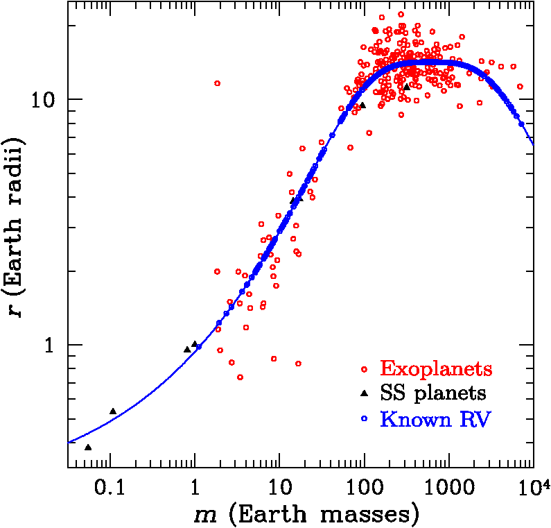

2.2.

Star Brightness

The host stars for the 127 RV planets in the present study all have a listed V magnitude, but are missing a blue magnitude minus visible magnitude (B-V) color, so this was supplied using the following empirical fit to data from Appendix C of Ref. 15:

To obtain the photon rate, we use the following empirical expressions, obtained from examination of the tables in Ref. 15 (Appendix C), and using the formalism for $f(\lambda ,m)$ in Ref. 16:

2.3.

Planet Brightness

The planet’s illumination geometry is estimated for a circular orbit, an average orbital inclination $i=60\mathrm{deg}$ with respect to an edge-on orbit, and an angular anomaly $\theta =70\mathrm{deg}$ in the plane of the orbit, measured with respect to superior conjunction. A circular orbit is chosen because the actual orbits are roughly circular, with a median eccentricity of 0.21. The inclination angle is chosen to represent the statistical average of the as-yet unknown inclination. The angular position is chosen to represent a point in the orbit where the planet is expected to be relatively bright and relatively far from its star, i.e., it is slightly brighter than at maximum elongation, and slightly closer to the star in angular separation. This orbital location gives a phase angle $\alpha$ specified by $\cos (\alpha )=\sin (i)\times \cos (\theta )$, or $\alpha =72.77\mathrm{deg}$, which in turn gives an angular separation on the sky of

The planet brightness is estimated for a visible geometric albedo of $p=0.50$, which is roughly the same as Jupiter’s albedo in the range of 400 to 700 nm, and representative of Jupiter’s continuum segments from 700 to 1000 nm, shown in Fig. 2. The planet’s phase function $\mathrm{\Phi }$ is taken to be a Lambert scattering function,

Fig. 2

Geometric albedo of Jupiter and Uranus,¹⁷ showing the albedo as a function of wavelength, the characteristic widths of spectral features (nearly all ${\mathrm{CH}}_4$), the four proposed filter locations and widths, and the three proposed spectrometer bands and resolution elements, drawn here at a resolution of $R=70$, chosen to approximately match the widths of the narrowest features in these spectra, and therefore maximize the accuracy of inferred ${\mathrm{CH}}_4$ mixing ratios.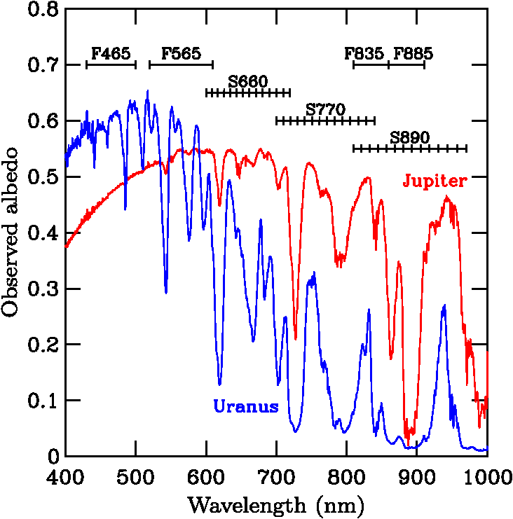

We show in Fig. 3 the estimated contrast of known RV planets, as a function of their angular separation as specified above, for the 127 RV planets that fall in the range of planet-star separation angles given above, i.e., $\beta >0.040\mathrm{arc}\sec$.

Fig. 3

Contrast versus angular separation for the 127 exoplanets in the RV catalog used in this paper, assuming circular orbits, $i=60\mathrm{deg}$ inclination, $\theta =70\mathrm{deg}$ orbital location, $p=0.50$ visible albedo, and Lambert phase function.

In this paper, we assume that the orbital period and phase are well known, allowing us to estimate the optimum calendar date on which to search for the planet. It is beyond the scope of this study to set requirements for the accuracy and frequency of precursor RV observations needed, and it is also outside the scope of this paper to carry out DRM studies to set requirements for the schedule of visits to a target, and the observational completeness (fraction of visits that result in a useful measurement). For a broad range of inclinations, with an up to date RV solution, it is possible to determine a range of dates over which the planet will have best observability (typically between 60 and 90 deg phase). The main remaining uncertainty is the position angle on the sky, which requires that the search range be able to cover 360 deg of azimuth, either in one observation or in sequential ones.

2.4.

Uncertainty in Planet Contrast and Angular Separation

In this section, we estimate the relative uncertainty in the expected star–planet contrast $C$ and star–planet angular separation $\beta$. This uncertainty is based on the planet-to-planet variations that might exist in nature, including albedo, diameter, eccentricity, and orbital orientation with respect to the observer; it is not an estimate of SNR, which we address in Sec. 4.10.

For RV planets, we already know the planet mass, semimajor axis, and eccentricity with a reasonable degree of accuracy. From these known values, we can estimate the planet radius and brightness, and the relative uncertainties in all quantities, as follows.

The contrast is a function of albedo, phase function, planet radius, and orbit radius, as given above, where the latter is given by

The relative uncertainty in contrast, $\mathrm{\Delta }C/C$, is given by the differential approximation

We now proceed to estimate each of the contributing terms in these two equations. For albedo, the observations of solar system giant planets by Ref. 17 are useful as a guide to what might be expected for the RV exoplanets, which are dominantly Jupiter-mass objects, with a median semimajor axis value of $\sim 3.3\mathrm{AU}$. Karkoschka measured the visual spectra of Jupiter, Saturn, Uranus, and Neptune in 1993 and 1995, with statistical and systematic accuracies of better than 1 and 4%, respectively. He found that the time variation of full-disk magnitudes in the V, R’, and I’ bands for these four planets was $\sim 0.012$ magnitudes rms, or $\sim 1.2\%$. The full-disk albedos in a continuum region at 550 nm, in a 15% band, are estimated from Karkoschka’s spectral plots to be $\sim 0.52$, 0.50, 0.60, and 0.54 (all times 1.05 to correct the values to full opposition) for Jupiter, Saturn (with the rings edge-on, so very little of the disk was shadowed), Uranus, and Neptune, respectively, giving an average of 0.567 and an rms scatter of $\pm 0.045$. The relative uncertainty in exoplanet albedo is therefore taken to be $\mathrm{\Delta }p/p\cong 0.079$.

We note that the albedo of a giant planet is expected to be as high as indicated above only for the case where the planet is sufficiently far from its star that water and ammonia clouds can form in the atmosphere. When the planet moves closer to its star, for example, for Jupiter, between $\sim 0.8$ and 2 AU from the Sun,¹⁸ these clouds tend to be absent, owing to the atmospheric temperature exceeding the condensation temperature, so the incident starlight will not be reflected, rather it will penetrate deeper into the atmosphere, and will tend to be absorbed by molecular features such as those of ${\mathrm{CH}}_4$, leading to a lower albedo for planets at these closer orbital radii (e.g., Ref. 2). We do not consider these lower albedos in this study because the inner working angle of the prime coronagraphs on WFIRST will preclude finding many such objects.

For the phase function $\mathrm{\Phi }$, the Lambert law is used, along with the relation for phase angle $\alpha$ in terms of orbital inclination $i$ (angle between orbital plane and observer’s sky) and angular anomaly $\theta$.

For the planet radius $r$, the median difference between the individual radius values and the smooth curve in Fig. 1 is $\sim 13\%$, giving $\mathrm{\Delta }r/r\cong 0.013$.

For the orbital radius $R$, we use the approximate relation

For the sine of the phase angle, we use the nominal angular anomaly $\theta$ and the range of inclinations to find $\mathrm{\Delta }\sin (\alpha )/\sin (\alpha )\cong 0.016$. For the observer-star distance $d$, we use the median uncertainty in distance to the above set of RV targets to find $\mathrm{\Delta }d/d\cong 0.008$. The combined result is a relative uncertainty in contrast of $\mathrm{\Delta }C/C\cong 0.39$ and an uncertainty in angular separation of $\mathrm{\Delta }\beta /\beta \cong 0.036$, as shown in Table 1. These values will be used in Figs. 8Fig. 9–10, where we plot the contrast versus separation for RV planets.

Table 1

Relative uncertainties in the contrast and separation of RV planets with respect to their parent stars, as estimated for the set of known RV planets accessible to the coronagraph on WFIRST. The contributing terms are also listed, for completeness.

The large gap between the uncertainties owing to the combined effects of albedo, phase function, and semimajor axis, versus the uncertainty from planet radius, suggests that photometric measurements of the contrast of directly imaged planets might be considered as evidence for planet radii, with the other parameters being inferred from the measured geometry of the system plus inferences of the planet albedo on the basis of model atmospheres, a possibility once suggested by Ref. 7, but shown here more quantitatively.

3.1.

Telescope Model

Our telescope model comprises the shape of the pupil (including the central obscuration and six spider arms), the off-axis angle of the CGI, the mirror prescriptions, the model power spectral density (PSD) of phase and amplitude errors of the primary mirror and secondary mirror, the model root-mean-square (RMS) pointing jitter, the coating reflectivity as a function of wavelength, and the polarization transformation as a function of wavelength and position within the pupil. In a separate calculation (not included in this paper, but relevant to our estimates of the time needed to create a dark hole), we use estimates of the model wavefront deformation owing to thermal changes in the shape and location of telescope mirrors, as a function of pointing angle, and recent slew angle history.

3.2.

Coronagraph Model

Our coronagraph model includes the two coronagraph architectures that were chosen as the prime instrument after a community-wide downselection process in 2013, plus a third architecture as a study-phase backup.¹⁹ The prime instruments are the HLC (Refs. 20 and 21) and the shaped pupil coronagraph (SPC).^22,23 The HLC and SPC are combined into a single package, the occulting mask coronagraph (OMC), in which operation in HLC or SPC mode is determined by the selection of a flip mirror. The backup instrument is the phase-induced amplitude apodization complex mask coronagraph (PIAACMC).^24,25

The coronagraph data files in this paper are all for 550 nm and 10% bandwidth. The HLC design is from Moody on September 15, 2015, which in turn is a slightly improved version of a design from Moody and Krist on August 14, 2014, with the name 20140623-139, for a single polarization. The SPC design is from Krist on September 25, 2014, labeled 20140902-1, for unpolarized light. The PIAACMC design is from Guyon and Krist on March 26, 2015, labeled 20150322, or Gen3, for a single polarization.

All these architectures are currently (early 2016) being developed in parallel in the lab. Each uses a combination of phase and amplitude control of the wavefront, in the pupil, near-pupil, and image planes, to achieve contrast values on the order of ${10}^{-9}$ over a range of azimuthal and radial angles on the sky. The coronagraph systems feed both a direct imager and an integral field spectrometer (IFS).²⁶

The status of the OMC in its lab testbed is that it has passed its scheduled milestones on time, including the most recent one (September 2015) of achieving a raw contrast of ${10}^{-8}$, with a bandwidth of 10%, at a central wavelength of 550 nm, in a static environment. Its next milestone (September 2016) is the same but in a dynamic environment, which will include pointing jitter of the telescope.

The status of the PIAACMC is that its focal plane mask with at least 12 concentric rings has been fabricated and characterized, and that the results are consistent with model predictions of ${10}^{-8}$ raw contrast, with a bandwidth of 10%, at a central wavelength of 550 nm, all of which was for its most recent milestone (December 2014). Its next milestone (September 2016) is to demonstrate a raw contrast of ${10}^{-8}$, with a bandwidth of 10%, at a central wavelength of 550 nm, in a static environment, and that its contrast sensitivity to pointing and focus is characterized.

In the present paper, we estimate coronagraph performance at wavelengths other than 550 nm, and bandwidths other than 10%, as specified in Ref. 1, and as will be displayed later in Table 2. We do this by scaling the 550-nm design by wavelength, assuming that the scaled designs can be implemented in the lab. We further assume that the 10% bandwidth can be extended to the bandwidths in Table 2, by appropriate design changes. Thus, the yield estimates in this paper are based on coronagraph designs that have yet to be created in the computer and implemented in the lab, but which we feel are achievable, based on past experience.

Table 2

Science filter bands. For each filter, the columns give the central wavelength, ratio of FWHM to central wavelength, nominal science purpose, polarization state, destination focal plane, and coronagraph architecture to be used for that filter and destination. The filters are as listed in the WFIRST-AFTA report,1 and as such are goals for technology development.

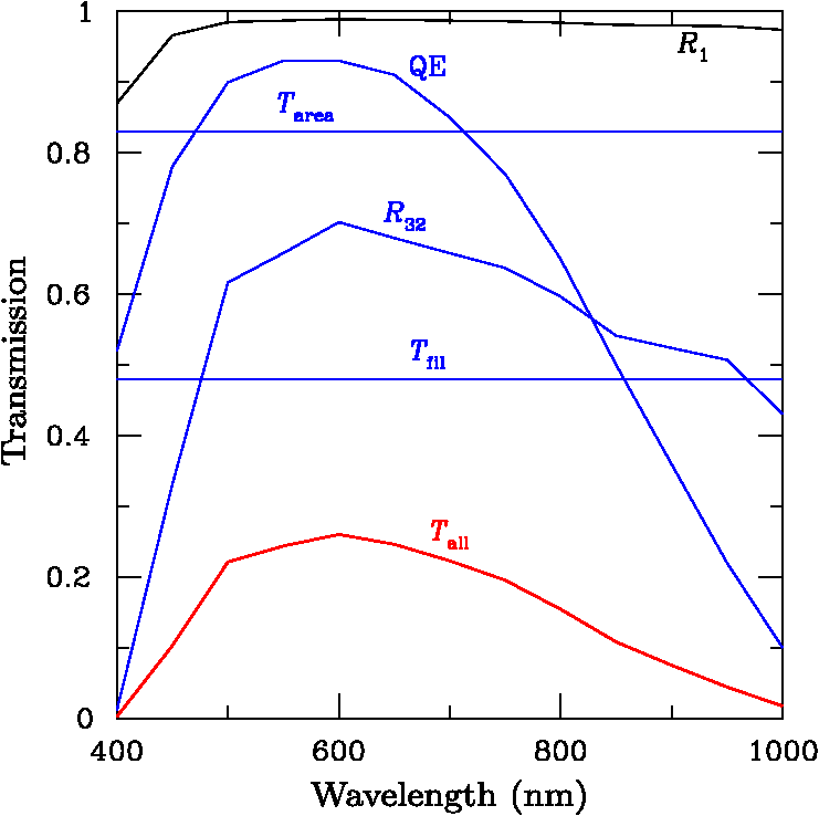
3.3.

Detector Model

Our detector model is based on the well-known electron-multiplying CCD201 (EMCCD) from e2v.²⁷ Model parameters include pixel size, wavelength dependence of quantum efficiency, and parameters for each of the three read modes: ordinary CCD-type operation (zero gain), electron-multiplying analog operation, and electron-multiplying photon-counting operation. All three modes are accessible during flight, but for the present estimate, we use only the latter, most sensitive, photon-counting mode. Key parameters of interest, as used in the current simulations, include dark current ($0.0005\text{electrons}/\mathrm{s}$ per pixel), clock-induced charge (0.001 electrons per pixel per read), gain factor (500), read noise (16 electrons RMS per read), and integration time per snapshot (300 s).

3.4.

Wavefront Propagation Model

Our wavefront propagation model is the PROPER program²⁸ employed for all of the instrument performance calculations in this section. PROPER propagates a scalar wavefront through all of the telescope and CGI optical surfaces, in the near and far fields, using Fourier-based Fresnel and angular spectrum methods. For the purpose of calculating science yield, the key results from PROPER are the azimuth-averaged contrast values of the background speckle field and the fraction of planet light in the core of the PSF as given by the area enclosed by the full-width at half-maximum (FWHM) of the focal-plane image of a point source on the sky. Values for these two parameters are calculated for each of the two orthogonal linear polarizations, as a function of radial angle on the sky, for (1) selected values of the RMS angular jitter of the telescope pointing direction, (2) a given PSD of polishing errors and amplitude errors on the telescope mirrors, (3) two values of the factor by which the speckle intensity can be reduced, and (4) the function integrated over the full wavelength band.

Polarization is accounted for by noting that the portion of the incident wavefront that is reflected from the angled mirrors (including the primary mirror) will suffer a phase delay between the radial and tangential components, which in turn negatively affects the coronagraph’s performance. Therefore, we currently plan to separate the $x$ and $y$ polarizations with a Wollaston prism placed immediately in front of the direct-imaging detector; the coronagraph deformable mirror settings can be tuned to optimize contrast in either $x$ or $y$ polarization. The spectrograph may use either a single fixed polarizer or none; simulations show the SPC is less sensitive to these low-order differential aberrations. Thus, the dark hole will be achieved and the science measurements taken in one or both polarizations, depending on the science goals, and in all cases, both polarizations will be simultaneously recorded.

4.1.

Transmission Factors Versus Wavelength

The wavelength-dependent instrument transmission factors, which are independent of the coronagraph, are shown in Fig. 4. Curve $R_1$ is the reflectivity of a single overcoated silver mirror, for a typical coating (FSS99-600, Ref. 29) at near-normal incidence. Curve $R_{32}$ is the reflectivity of 32 such mirrors, i.e., $R_{32}=R_1^{32}$, where the value of 32 is from a recent stage of design of the CGI. The curve QE is a typical quantum efficiency of the CCD201-20 detector at $-20°\mathrm{C}$, with a midband coating (e2v data sheet). The curve $T_{\text{area}}$ is the geometric transmission factor of the telescope’s spiders and central obscuration, compared to a 2.4-m clear aperture. The $T_{\text{fil}}$ curve is an estimated transmission factor comprising the nonsilver elements of the optical train, including the reflectivity of two deformable mirrors at 93% each, two focal plane mirrors at 97% each, and one color filter at 60% transmission. The $T_{\text{all}}$ curve is the product of all the above transmission factors.

This transmission factor is independent of a coronagraph’s diffraction terms, listed in Sec. 4.2.

Fig. 4

Transmission factors for the coronagraphs on WFIRST, showing the wavelength dependence of quantum efficiency and mirror reflectivity, and the nominal wavelength independence of the secondary blockage and filter terms.

4.2.

Transmission Factors Versus Angle

There are three types of star-planet angle-dependent transmission factors to be considered for each coronagraph design, as shown in Fig. 5 for HLC, SPC, and PIAACMC. These are the solid-angle factor $\mathrm{\Omega }$ ($\mathrm{arc}{\sec }^2$), a point-source transmission factor $T_{\text{point}}$, and a diffuse-source transmission factor $T_{\text{diffuse}}$. In the present study, we assume that a single polarization of light is selected prior to detection for the HLC and PIAACMC coronagraphs, for the reason that the contrast is degraded by a factor of at least 3 or 4 for unpolarized light compared to linearly polarized light, which is not acceptable. On the other hand, for SPC, the factor is a more modest 1.5 to 2.0, which is more acceptable.

Fig. 5

Transmission factors for all three coronagraphs, as a function of planet–star separation. The design wavelength is 550 nm, so for other wavelengths, the planet–star axis must be scaled proportional to wavelength. The bottom group, $\mathrm{\Omega }$ (square arc-second, ${\mathrm{as}}^2$), is the projected solid angle on the sky of the FWHM of the PSF. The middle group, $T_{\text{point}}$, is the transmission factor for point sources, and the upper group, $T_{\text{diffuse}}$, is the transmission for a diffuse source, here the solar system zodi. The $T$ values are for single polarization for HLC and PIAACMC, and unpolarized light for SPC.

The upper scale in Fig. 5 indicates the planet–star separation in units of $\lambda /D$, where $\lambda =550\mathrm{nm}$ is the design reference wavelength and $D=2.37\mathrm{m}$ is the design reference telescope diameter, so that $\lambda /D=1$ is an angle of 0.04787 arc sec. For other wavelengths, we scale the curves in Fig. 5 by $\lambda$, so, for example, at longer wavelengths, the curves shift toward larger angles in arc sec units, and the PSF area increases (as ${\lambda }^2$). We discuss the resulting transmission factors in the present section.

4.3.

Speckle Contrast Versus Angle

As a wavefront of a given photon passes through the optical system, it encounters (polarization-dependent) transverse variations of phase and amplitude, and each Fourier component of these variations gives rise to the probability that the photon will end up being diffracted in a direction outside the nominal solid angle $\mathrm{\Omega }$ where the point-source-like image is located. These diffracted photons form a distribution of faint pseudo images across the dark hole, which we call speckles.

In the present simulation, the intensity and spatial distribution of speckles is estimated by assuming, from experience, a PSD, which describes the phase and amplitude distribution, in a statistical sense. We further assume that the deformable mirrors are driven to scatter additional starlight onto the locations of these speckles, but with an opposite phase, thus canceling the net electric field at each point in the dark hole to the maximum extent possible. The resulting speckle intensity is then averaged in azimuth, giving the speckle–star contrast factor $C_{\text{spec}}$ as a function of planet–star separation, and shown for each coronagraph in Fig. 6.

Fig. 6

Contrast of speckles in the dark hole for each coronagraph, for a small residual jitter (0.4 mas RMS) and a large residual jitter (1.6 mas RMS), at the design wavelength of 550 nm. For other wavelengths, the planet–star angle is replaced by one that is wavelength scaled, as suggested by the $\lambda /D$ axis at the top.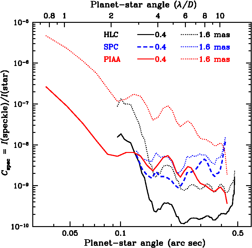

A second factor that is taken into account in Fig. 6 is spacecraft pointing jitter. It is known that momentum wheels have slightly imperfect balance, so that as they rotate, even at constant angular speed, the spacecraft moves in opposition, resulting in a variation of the space direction of the optical axis of the telescope, with a frequency equal to that of the wheel. In addition, the spacecraft structure can respond in its resonant modes, resulting in additional pointing errors. The net result is that a star image will be displaced with respect to its intended position, and some extra light will leak past the coronagraph. The situation is simulated by summing the results of a distribution of stellar offsets. See Ref. 31 for a discussion of the expected pointing jitter amplitudes and frequencies, and Ref. 28 for a discussion of the speckle simulations. We assume that the intrinsic jitter level of the spacecraft is 14 mas RMS per axis, with a Gaussian distribution. The motion of the star image is suppressed by a low-order wavefront sensing and control system,³² resulting in a residual, uncompensated jitter level that is expected to be bounded by $\sim 0.4\mathrm{mas}$ RMS at the low end, and by $\sim 1.6\mathrm{mas}$ RMS at the high end. Note that the star is assumed to have a diameter of 1.0 mas (e.g., the Sun at 10 pc), which means that it is not worthwhile to suppress the pointing jitter to much less than 0.5 mas RMS.

In this paper, the expected speckle contrast levels $C_{\text{spec}}$ for two bounding cases are shown in Fig. 6 as thick lines for the good (0.4 mas) case and as thin lines for the bad (1.6 mas) case. Notice that the good and bad cases are separated by about a factor of 2.5 for the SPC, indicating that it is relatively immune to pointing jitter. The good and bad cases for HLC are separated by a factor of $\sim 7$, and for PIAACMC, the separation is about a factor of 20, indicating increased sensitivity to uncompensated pointing jitter.

In Fig. 6, as in Fig. 5, the curves for $C_{\text{spec}}$ are drawn for 550 nm and 2.37 m diameter, so for longer wavelengths, for example, the curves shift to larger values of angle in arc sec units. The practical effect is that for longer wavelengths, we lose the ability to measure planets at smaller angles, but gain an ability to see planets and disks that might lie at larger angles from the star.

4.4.

Target Count Rates

We start by estimating the count rate $n_{\text{star}}$ (electrons per second) from a target star of magnitude $m_{\text{star}}(\lambda )$. If the telescope is pointed slightly away from the target star, so that the star falls within the area where the dark hole would normally be located, the count rate from the star will be

The planet count rate $n_{\mathrm{pl}}$ is then given by the count rate of the star times the contrast factor ($\text{planet}/\text{star}$), from above, giving

4.5.

Background Count Rate from Zodiacal Light

The total background count rate from the sky is the sum of intensities from speckles and local zodi plus exo-zodi, in this section. (In this study, we ignore scattered and diffracted contributions from companion stars.)

For a representative value, we define one zodi to have a brightness of

For the current simulation, we assume that the solar system zodi brightness is a factor ${\mathrm{num}}_{\mathrm{ss}}=1$ times brighter, giving a count rate in the focal plane of

For the external zodi, we use a model adopted by Ref. 33 from a numerical simulation by Kuchner (Ref. 34, Appendix A), which gives the brightness as

Using the relation for the magnitude $m_{\text{ext}}$ of the external zodi, we find that the count rate $n_{\mathrm{ext}1}$ in the focal plane, for a zodi disk identical to the solar system disk, is

4.6.

Condition for Disk to Match Planet

It is of interest to ask, for each RV planet, what disk brightness is needed to make the disk signal equal the planet signal? Knowing this value will give us an idea of (1) how much disk background can be tolerated before the planet signal begins to be obscured by the disk, as well as (2) how bright a disk we can expect to detect around a star similar to the RV target star, given that we already have established that we could detect a planet around that star. We reserve for a future study an analysis of disk detection in the general case.

Let ${\mathrm{num}}_{\text{equiv}}$ be the equivalent number of zodis needed in order for the disk signal to equal the planet signal. Using the results of Secs. 4.4 and 4.5, we find

4.7.

Background Count Rate from Speckles

The count rate $n_{\text{spec}}$ from speckles, in the FWHM solid angle $\mathrm{\Omega }$ on the detector, is given by

For the present study, a much more detailed simulation was performed, using expected values of surface (phase) and reflectivity (amplitude) errors of all optical elements, additional wavefront distortions owing to polarization effects, and an estimate of how well the deformable mirrors could correct the net phase and amplitude errors of the propagated wavefront. At each angular distance from the star, the resulting scattered light intensity in the focal plane was averaged over azimuth angle and expressed as a contrast value as a function of angular radius. Given that the spatial RMS variation of speckles is approximately equal to the average speckle intensity, this resulting intensity distribution is treated as a background noise, against which the planet intensity is to be measured.

4.8.

Total Count Rate

The total number of detectable electrons per second from the sky, $n_{\text{sky}}$, in the solid angle $\mathrm{\Omega }$ is the sum of the planet ($n_{\mathrm{pl}}$), solar system zodiacal light background ($n_{\text{ssz}}$), external zodi level ($n_{\text{ext}}$), and speckle background ($n_{\text{spec}}$) count rates:

The total measured number of electrons per second is the sum of the detected sky rate (above) plus detector contributions. An expression that includes CCD-type detectors as well as electron-multiplying CCDs²⁷ is as follows:

Table 3

Astrophysical and instrumental parameters, and typical values, for detecting a typical exoplanet with the CGI on WFIRST, for CCD and EMCCD detectors, and the resulting integration times.

4.9.

Noise Count Rates

The noise in a measurement is contributed by two main sources: (1) statistical fluctuations in the number of measured electrons and (2) the uncertainty in subtracting the background, where the background can vary spatially (e.g., zodiacal light and speckles) and vary with time (e.g., speckle brightness changes owing to thermally induced optical path variations in the telescope). Our ability to reduce this noise is limited by the nature of the fluctuations and by the effectiveness of our postprocessing algorithm.

For noise source 1, the RMS noise $N_1$ (elec) after a total integration time $t$ is

The statistics of speckles tells us that the spatial RMS variation in intensity is equal to the average value of the speckle intensity. The expected thermal variations of the optical paths within the telescope and coronagraph tell us that there also will be a time-varying component of speckle intensity. Using experience from ground and space observations, we expect that the total RMS variation could be reduced by postprocessing, by a factor $f_{\mathrm{pp}}$, where $f_{\mathrm{pp}}=1/10$ is our adopted worst-case estimate, and $f_{\mathrm{pp}}=1/30$ is our adopted best-case estimate. So for noise source 2, the RMS noise $N_2$ (elec) after a total integration time $t$ is

Adding these statistically independent noise sources gives us the total noise, after postprocessing, at the location of a planet, as

4.10.

Signal-to-Noise Ratio

The signal that we care about is $S_{\mathrm{pl}}$, the number of collected electrons from the planet, in the total integration time $t$, where

The ratio SNR of signal electrons to noise electrons is then

We adopt a detection criterion of a threshold SNR of a value of 5, so that

Solving for the total integration time $t$, we find

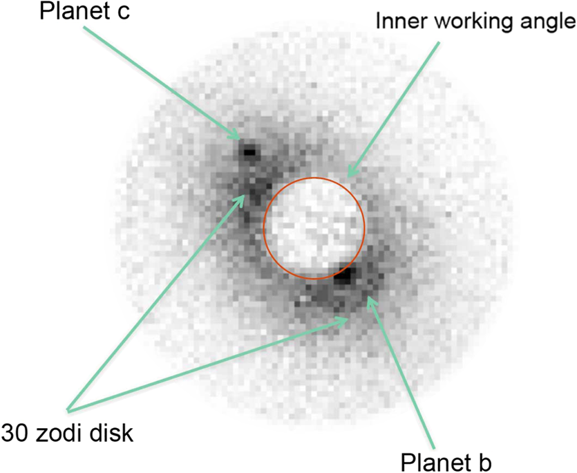5.1.

Hybrid Lyot Coronagraph Results

The science-imaging yield of known RV planets that are detectable with the HLC, in the 565-nm band (15%), for a single polarization (triangles), is shown in Fig. 8. The short-dash line (lower curve) is the 5-sigma speckle noise detection floor for the best case, which is a telescope pointing jitter of 0.4-mas RMS residual uncorrected angle, and a postprocessing factor of 30 times reduction in the spatial RMS speckle noise. The worst case (upper long-dash line) is similar, but for a pointing jitter of 1.6 mas and a postprocessing factor of only 10. The HLC has a 360-deg azimuth field, in a single snapshot. The IWA and OWA are effectively set by the angle limits of the floors as plotted. The solid triangle symbols are detections that can be carried out with the worst-case floor (upper); the open triangles are the extra planets that are detectable for the best-case floor (lower). For the HLC case shown, we expect to image about 15 RV planets, in a total integration time of 3 days, with an SNR of 5.0, in a single polarization, in this band, with an integration time of less than a day for each planet.

Fig. 8

Science imaging yield of known RV planets with HLC. Solid symbols are RV planets detectable with HLC in a 15% band centered at 565 nm, in less than a day each, in a single polarization, with a signal strength greater than the worst-case floor (long-dash line, 1.6 mas RMS pointing jitter, and a postprocessing factor of 1/10). The open symbols are for the additional detections possible with the best-case floor (0.4 mas jitter, 1/30 factor). Typical relative uncertainties in contrast and separation (Sec. 2.4) are indicated.

5.2.

Shaped Pupil Coronagraph Results

The science-imaging yield of RV planets with the SPC is shown in Fig. 9. Here the science yield is 15 RV planet detections, each of which could be done in less than a day if the position angle of the planet was known. However, because it is not known, and because the SPC can only observe an azimuth range of $\sim 120\mathrm{deg}$ per snapshot, it will take three such snapshots to cover the full azimuth range; therefore, the total observing time will be about 8 days. Once a planet is discovered, the SPC can then be set at an appropriate azimuthal orientation for subsequent snapshots, either to improve the SNR or to observe at a different wavelength. Another difference with respect to the HLC is that the SPC has a higher contrast floor, which will reduce the number of detectable planets when searching for new discoveries, which are fainter than the RV planets indicated. A compensating factor is that the SPC is less sensitive to telescope jitter, which gives it a better performance margin in flight. Another compensating factor is that the SPC is less sensitive to polarization effects, so both polarizations can be observed simultaneously. The baseline for WFIRST-AFTA is to use the HLC for initial discovery at short wavelength and the SPC for long-wavelength characterization, even though Fig. 9 shows the SPC at a shorter wavelength, for the sake of uniformity in this paper.

Fig. 9

Science imaging yield of known RV planets with SPC. Solid symbols are RV planets detectable with SPC in a 15% band centered at 565 nm, in less than a day each, in both polarizations simultaneously, with a signal strength greater than the worst-case floor (long-dash line, 1.6 mas RMS pointing jitter, and a postprocessing factor of 1/10). The open symbol is for the additional detection possible with the best-case floor (0.4 mas jitter, 1/30 factor). Typical relative uncertainties in contrast and separation (Sec. 2.4) are indicated.

5.3.

PIAACMC Results

The science imaging yield of the backup architecture, the PIAACMC, is shown in Fig. 10. This architecture has the advantage (Figs. 5 and 6) of a greater overall throughput as well as a theoretically smaller IWA, allowing it to access more planets close to their star. However, an accompanying disadvantage is that it is more sensitive to telescope jitter, which in combination with the adopted values of jitter produces higher 5-sigma floor contrasts, as indicated in the figure. Therefore, many planets that were detected by a large contrast margin with the HLC or SPC are now closer to the PIAACMC contrast limit and will therefore require the best possible operating conditions (lowest jitter and most aggressive postproduction factor). Also, this version of PIAACMC has only one deformable mirror; hence, the azimuthal field is 180 deg, so two snapshots are required in order to fully examine a new system. The higher throughput and smaller IWA result in a greater number of detectable RV planets, and at a faster rate per planet than for the HLC or SPC, but operating with a relatively smaller margin.

Fig. 10

Science imaging yield of known RV planets with PIAACMC. The solid symbol is for the single RV planet detectable with PIAACMC in a 15% band centered at 565 nm, in less than a day each, in a single polarization, with a signal strength greater than the worst-case floor (long-dash line, 1.6 mas RMS pointing jitter, and a postprocessing factor of 1/10). The numerous open symbols are for the additional detections possible with the best-case floor (0.4 mas jitter, 1/30 factor). Typical relative uncertainties in contrast and separation (Sec. 2.4) are indicated.

5.4.

Top-Ranked Radial-Velocity Planets

All RV planets in Figs. 8Fig. 9–10, with angular separations $>0.10\mathrm{arc}\sec$, are listed in Table 6. Explicit planet names, masses, radii, periods, and semimajor axes are listed, along with host star magnitudes. Each planet’s separation and contrast at a phase angle of 72.77 deg is listed, as discussed in Sec. 2.3. For the 565-nm band, the integration times for each of the HLC, SPC, and PIAACMC coronagraphs are given for each detectable planet.

Table 6

All detectable RV planets with angular separations >0.10  arc sec, in the 565-nm band, for each coronagraph. The integration times are in days. The ordering is from large to small separation angles.

8.1.

Time for Photometry of Known Radial-Velocity Planets

The total time required for a first-time detection of an RV planet is determined in this study by the integration time assuming that the planet is in an approximately optimum orbital position. It is likely that we can predict the right time to observe an RV planet because we already will have the ephemeris from RV observations, with only the inclination of the orbit and the position angle as unknown factors. For the current work, we assume a statistical average inclination of 60 deg. For HLC, with a full 360 deg of azimuth in a single snapshot, only one snapshot of a target needs to be taken. Numerical simulations show that all of the RV planets can be detected on the first try if they are observed when they are in the orbital range from $\sim 45$ to 90 deg, where 90 is maximum elongation. This range occurs $\sim 25\%$ of the time, allowing for orbital symmetry. Most RV periods are in the range of 2 to 10 years, so the time when a planet is in an optimum orbital window is easily predicted, assuming that ongoing Doppler measurements continually refine the orbital solution. The 40 days of clock time listed in the top part of Table 8 includes multiple filters and polarizations, as well as search time for the initial acquisition of the planet, and additional time to achieve better than the minimum SNR.

8.2.

Time for Spectra of Known Radial-Velocity Planets

We use SPC and IFS for spectra in the 660-, 770-, and 890-nm bands, at a spectral resolution of $\sim 70$, an ${\mathrm{SNR}}_0$ value of 5, and assuming that the albedo in the near-continuum regions is the same value (50%) as at shorter wavelengths. An integration time limit of 1 week is assumed for spectra, greater than the 1-day limit for filter photometry, owing to the higher spectral resolution. Two factors govern the yield of spectra: first, the IWA moves outward as the wavelength increases, cutting off planets that are too close to their star; second, the quantum efficiency of the detector decreases at longer wavelengths. The net result is that we expect to obtain spectra of RV planets at the rates of $\sim 11$ spectra in 30 days in the 660-nm band, 6 spectra in 17 days in the 770-nm band, and 1 spectrum in 6 days in the 890-nm band. All SPC spectra will be in the unpolarized mode.

8.3.

Time for Disk Images

As noted in Sec. 7, disks are automatically included in the search for RV planets, adding no extra time for that aspect. However, we expect to conduct a deeper search for disks around some of the RV target stars as well as additional targets, for which we allocate 30 days of observing time, subject to a future study.

(1) For as-yet-undiscovered (new) planets, a precise estimate of search time requires a full DRM, which will be carried out in future phases. We initially allocate 85 days for this search. (2) The WFIRST mission allocates $\sim 25\%$ of the time to a GO program, so for CGI, this would be 91 days. (3) We assume that we will need 1 day to set up the dark hole for each RV planet when observed for the first time. Then, for a given RV target, subsequent observations in a different polarization and with different filters should take less time to tune the dark hole, for which we assume a quarter-day each for $\sim 140$ targetings. We also assume that the initial checkout of the spacecraft will consume 5 days of coronagraph time. We thus conservatively estimate a total of 56 days of overhead.

8.4.

Total Time

Adding the aforementioned time allocations for CGI, we find a total of 365 days required for the proposed program, as shown in Table 8.

Table 8

Nominal time allocation and performance against requirements for CGI, for each major category of observation. These values will be updated when detailed engineering overhead times are available, and a realistic DRM can be calculated.